Understanding High-Volatility Stocks: Mean-Reversion and Trending Behavior
Some stocks look like they’re trying to win a speed contest—spiking, snapping back, then sprinting in the opposite direction a few hours later. That’s what people usually mean by high-volatility: prices that swing around a lot, often within relatively short windows. But the confusing part is this: high volatility doesn’t tell you whether the stock will keep pushing in one direction (trending) or keep returning to some “fair” level (mean reversion).
In practice, high-volatility behavior comes from a mix of market mechanics (liquidity and order flow), information timing, and who is trading. Once you see that, things get less mystical. You can start identifying when a stock is likely to behave like a rubber band and when it’s more like a train that doesn’t want to stop.
This article explains the statistical and structural reasons behind mean-reverting versus trending behavior in high-volatility stocks, and what that means for analysis and risk management. We’ll keep the background simple, but we’ll still talk like adults—because markets don’t care about vibes, they care about orders.
What “High Volatility” Actually Means (Beyond the Obvious)
Volatility is often described casually as “uncertainty,” but that’s not the best definition. In markets, volatility is usually a statistical measure: how much returns vary around their average. A stock can be volatile because it’s reacting strongly to new information, because capital flows are aggressive, or because liquidity doesn’t cushion shocks well.
Common measures include:
- Standard deviation of returns: How widely returns deviate from the mean.
- Average True Range (ATR): A practical gauge of typical price movement.
- Implied volatility (options): Volatility “priced in” by options markets.
The important point: volatility by itself doesn’t choose a direction. A stock can have large swings and still repeatedly mean-revert, or it can swing widely while trending because the swings come from ongoing directional order flow.
So when you look at a chart and think, “This thing is all over the place,” you’re not wrong—but you still need to ask a better question:
Is the stock’s movement dominated by tendency to return to an average level, or by persistent directional pressure?
Mean-Reversion vs. Trending: Not Just Two Vibes
The distinction between mean-reverting and trending behavior is structural. Each reflects a particular interaction among:
- Information flow (how quickly and how clearly markets update expectations)
- Liquidity conditions (how easily shares can be bought or sold without big price gaps)
- Order flow persistence (whether buying/selling pressure is one-off or repeated)
- Participant positioning (whether institutions are accumulating gradually or traders are flipping fast)
- Market regime (whether the broader environment encourages range trading or directional follow-through)
When those inputs lean one way, mean reversion tends to show up. When they lean the other, trending takes the wheel.
The Statistical Foundation of Volatility
Let’s make the math-friendly version of the concept. If a stock’s price frequently deviates from a central reference—like a moving average, VWAP, or an implicit equilibrium estimate—then volatility is high. The deviation itself might happen because the market overshoots temporarily, or because new information keeps shifting expectations.
From a statistical perspective:
- If deviations get “pulled back” over time, you get mean-reverting behavior.
- If deviations keep expanding because the drift is persistent, you get trending behavior.
In high-volatility stocks, either outcome can occur. A common misunderstanding is assuming volatility automatically implies randomness. Sometimes it is random noise. Other times, it’s noisy but structured movement—like a runner who stumbles right before clearing a hurdle.
The Fundamentals of Mean-Reversion
Mean-reversion is the idea that asset prices tend to move back toward an average over time. The “average” might be a moving average, a volume-weighted level like VWAP, or a statistical baseline derived from historical behavior.
In high-volatility stocks, you often see mean reversion when prices overshoot equilibrium due to short-lived imbalances. The overshoot can be caused by aggressive order bursts, algorithmic entry triggers, or sudden changes in how participants interpret information. After the initial shock, liquidity and profit-taking help pull the price back.
Mean reversion typically comes from a few overlapping dynamics:
- Short-Term Overextension: A big buy or sell sequence can push price beyond what current information justifies.
- Liquidity Provision: Liquidity providers may step in when price strays far, helping it move back toward a more “normal” trading zone.
- Statistical Arbitrage: Quant funds look for deviations from historical relationships and trade for corrections.
- Profit-Taking Behavior: Traders often close positions after sharp moves, which reduces momentum and encourages reversion.
Overreaction to Information
One of the most common reasons for mean reversion is the initial reaction to new information. Earnings, guidance, regulatory news—whatever the trigger is—can cause a fast price adjustment. But the first adjustment doesn’t always equal the eventual interpretation.
Early moves often overshoot because:
- Algorithmic trading triggers move quickly, before slow human confirmation arrives.
- Speculators and momentum traders pile in right away.
- Order imbalance is temporary even if the underlying story is stable.
As participants digest the information more thoroughly, prices can stabilize closer to a rational valuation band. In high-volatility names, that “overshoot then correct” pattern can repeat frequently.
Technical Anchoring Mechanisms
Mean reversion can be reinforced by technical reference levels. Indicators and chart levels aren’t magic, but they’re widely watched. When enough traders put their money near these levels, they become self-referential.
Examples include moving averages, Bollinger Bands, pivot points, and prior day highs/lows. If a stock drifts outside a commonly monitored band, traders may enter countertrend positions—turning statistical reversion into something closer to a tradable rhythm, especially in liquid high-volatility stocks.
Role of Market Microstructure
Mean reversion isn’t just psychology; it’s also plumbing. Market microstructure—the way orders match, how spreads change, and how venues fragment trading—strongly influences reversion patterns.
In a highly liquid stock:
- Depth in the order book can absorb shocks more smoothly.
- Price gaps are smaller and more likely to be corrected as liquidity replenishes.
In a thinly traded stock, shocks can overshoot for longer simply because there aren’t enough resting orders to provide a stabilizing counterbalance. That can delay reversion—or, if the imbalance persists, flip the behavior into trending.
The Nature of Trending Stocks
Trending behavior appears when directional order flow persists. Prices move upward or downward with limited retracement because the market keeps receiving bids (or offers) strong enough to maintain drift.
High-volatility stocks can trend hard when new information materially changes expectations or when capital allocation decisions motivate sustained buying or selling. The chart then looks less like a bouncing rubber ball and more like a conveyor belt.
Trending patterns often show the following traits:
- Persistent Institutional Flow: Funds accumulate or distribute across multiple sessions.
- Breakout Confirmation: When price clears notable levels, more participants join.
- Repricing Events: Structural updates (product changes, regulation, guidance) alter expected cash flows.
- Momentum-Based Trading: Quant models allocate capital to winners, which can amplify the trend.
Fundamental Catalysts and Structural Change
When trends persist, it’s often because expectations changed in a way that doesn’t easily revert. For instance, a company might report sustained margin improvements, or a regulatory decision might reduce previously perceived risk. If investors revise earnings models broadly, price has room to move and room to keep moving.
In those cases, the market isn’t merely correcting an overreaction; it’s repricing. Mean reversion expects a “pull back” toward a stable average. Trending happens when the average itself shifts.
Sector and Macro Influence
Stocks rarely respect your individual chart. Sector-wide repricing can cause synchronized directional movement. If interest rate expectations move, financials may revalue. If commodity prices shift, energy and materials often follow.
Macro alignment also matters. High-volatility in a stock is sometimes just the stock’s way of reflecting bigger forces loudly. When the macro story stays consistent for a while, trending becomes more likely because the flow doesn’t fade quickly.
Technical Breakouts and Momentum Reinforcement
Technical breakouts can turn an initial move into a longer trend. When price passes a widely watched resistance or support level—especially with rising volume—traders interpret it as confirmation.
Then you get feedback:
- Breakout traders enter.
- Systematic strategies add exposure based on signals.
- Stops get triggered on the other side, forcing additional buying/selling.
This is one reason why high-volatility names can suddenly sprint after being choppy for hours. The “chop” often ends when the market believes the direction is real enough to act on.
Market Conditions and Regime Shifts
Whether a high-volatility stock mean-reverts or trends depends heavily on the broader environment. Traders talk about “regimes” for a reason: the behavior of liquidity and risk appetite changes.
A simple way to think about regimes is by their effect on two things:
- Liquidity distribution: where liquidity sits and how easily it gets replenished
- Risk appetite: whether participants chase direction or prefer selling strength/buying weakness
Low-Confidence Environments
When uncertainty is high, participants may avoid extended directional commitments. They take profits quickly, reduce exposure, and keep trading inside well-defined boundaries. That creates a range-like stampede: price oscillates because the market doesn’t reward holding through noise.
In these conditions, high volatility can still look “organized” because mean reversion becomes the dominant behavior.
Directional Confidence Phases
When confidence increases—perhaps due to clear earnings trends, easing macro fears, or regulatory clarity—participants hold direction longer. Retracements shrink because funds don’t want to sell a trend they expect to continue. Here, volatility increases while pullbacks remain comparatively shallow.
Volatility Clustering
There’s a well-known empirical pattern: volatility clusters. High-volatility periods often follow high-volatility periods. But clustering doesn’t guarantee mean reversion or trending on its own.
It just says the market is likely to stay “excitable.” That excitability can produce either:
- Range-bound swings with corrections (mean reversion), or
- A widening drift supported by systematic flows (trending).
The missing ingredient is whether order flow persists directionally or rebalances around equilibrium.
Behavioral Influences on Price Patterns
Behavior doesn’t replace microstructure and statistics, but it explains the human side of why the same stock can behave differently at different times. Behavioral finance points out recurring tendencies in decision-making.
Herding Behavior
When traders see price move, they often treat movement as information. If other participants pile in, momentum becomes self-reinforcing. That can amplify trending behavior, especially when benchmarks and performance incentives make participation attractive.
For high-volatility stocks, herding tends to show up as a sudden shift from chop to directional movement after a threshold is crossed.
Loss Aversion and Reversion
Another behavioral factor is loss aversion. Traders often dislike being wrong and may exit positions quickly after sharp moves against them—particularly intraday.
That behavior can create frequent reversals and raise the odds of mean reversion during active sessions. It’s not always rational, but markets have never paid for rationality on a receipt.
Anchoring Effects
Anchoring means people rely on prior references. In trading, those references become:
- prior highs/lows
- previous day settlement
- round-number levels
- moving averages
As price approaches those anchors, trading activity often increases. Depending on whether more participants want to buy or sell at that level, price may consolidate or revert to the anchor.
Time Horizon Considerations: The Same Stock, Different Stories
The distinction between mean reversion and trending can depend on timeframe. A stock might trend intraday but revert over a longer period—or the reverse. This happens because the drivers of price differ across horizons.
Intraday Dynamics
Intraday price action is heavily shaped by high-frequency trading, algorithms, and rapid shifts in order book liquidity. Short-lived imbalances often produce mean reversion at the micro level.
However, if order flow remains unbalanced—say, due to persistent buying from a larger buyer or continuous demand from systematic strategies—directional runs can still dominate within the same session.
Multi-Day and Weekly Trends
Over days and weeks, institutional activity becomes more apparent. Portfolio rebalancing takes time. Execution schedules smooth out minute-level noise, allowing directional effects to persist.
So a stock that mean-reverts during the day might still trend in a higher timeframe because the underlying position changes are directional and slower to unwind.
Liquidity and Participation Structure
Liquidity affects both how large price moves become and how quickly the market corrects them. Depth and spread dynamics are a big deal in high-volatility names because “thin” stocks can exaggerate movement.
Institutional Versus Retail Participation
Participation often determines behavior. Stocks with higher institutional ownership can show more structured trending because institutions tend to trade systematically and over longer windows. Conversely, stocks dominated by short-term retail participation may show sharper spikes followed by quick reversals because participants react rapidly and exit quickly.
This isn’t a moral judgment. It’s a trading rhythm issue.
Regime Detection: When Analysts Try to Turn Guesswork Into Filters
If you’re actively trading (or even just trying to avoid stepping on your own rake), you need a process for identifying behavior regimes. Many traders use quantitative filters to decide whether to treat the market as mean-reverting or trend-prone.
Common indicators and statistical tools include:
- Average Directional Index (ADX): Estimates the strength of directional movement.
- Hurst exponent: Helps estimate persistence versus mean-reverting behavior statistically.
- Volatility contraction/expansion metrics: Identify transitions between tighter ranges and breakout-like expansion.
No single metric perfectly classifies behavior. But combining them can reduce obvious mistakes, like applying mean-reversion tactics during a genuine repricing trend where the “average” has shifted.
Interaction Between Mean-Reversion and Trend Phases
High-volatility stocks rarely do only one thing forever. Markets cycle. You’ll often see patterns that look like:
- mean-reverting consolidation
- followed by a breakout into trend
- then later, exhaustion and return to range behavior
That cycling happens because liquidity conditions and order flow persistence change over time.
Compression Before Expansion
A common sequence is compression (tighter price fluctuation) followed by expansion (wider moves). During compression, price often oscillates around a local equilibrium because order flow is balanced.
When a new catalyst emerges—earnings surprise, guidance clarity, contract announcement, macro data—the imbalance increases. At that point, mean-reverting pressure weakens, and trending begins because the market now has a reason to reprice more persistently.
Exhaustion and Rebalancing
Trends eventually run into limits. Buyers or sellers reach position constraints, and marginal participants may stop adding exposure. Once that happens, the trend loses momentum.
After exhaustion, the stock can shift into a phase where price moves away from a developing average and then corrects—more mean-reverting than trending. Even within broader bull or bear trends, short cycles of mean reversion often appear as the market digests new information and rebalances risk.
Macro Events and Structural Volatility Drivers
Macro events don’t just move whole sectors; they also change how participants trade. Interest rate changes, geopolitical developments, and fiscal policy updates can add layers of uncertainty or clarity.
High-volatility stocks are especially sensitive because they often have:
- greater expectations embedded in valuation
- more leveraged balance sheets or growth assumptions
- higher sensitivity to risk premiums
In macro-driven expansions, correlations often rise. When many stocks move similarly, the market receives persistent directional signals, which strengthens trending behavior.
But in uncertain macro transitions, directionality can fragment. Different stocks may react differently to the same headlines, and the resulting participation can promote broader mean-reverting behavior as traders adjust and re-adjust.
Practical Examples: How This Shows Up on Real Charts
Some of this stuff sounds theoretical until you watch it happen. Here are a few real-world patterns traders often recognize.
Example 1: Earnings Day “Overshoot Then Settle”
Picture a stock that releases earnings after the close. The next morning it gaps up 8–12% on strong results. If the initial move overshoots—because traders interpret the news too aggressively—price may later drift back toward a VWAP-like reference or a moving average.
During that drift, you’re likely seeing mean reversion driven by:
- profit-taking after the early spike
- liquidity providers stepping in as price gets stretched
- quant strategies reducing exposure after deviations
Example 2: “New Narrative” Trend After Guidance Clarity
Another possibility is that the company provides guidance that changes the narrative. Market participants revise their long-term model and adjust risk assumptions. In that case, price may not just overshoot; it may reprice and keep repricing.
Here, trending behavior appears because the market average is shifting. Retractions may happen, but the overall drift remains directional for days or weeks.
Example 3: Choppy Name in Calm Markets, Trends During Macro Stress
A high-volatility stock might look like it mean-reverts during calm periods: it spikes, then corrects within a consistent band. Then a major macro announcement hits or an unusual event changes risk appetite, and suddenly the same stock starts trending.
That shift usually means:
- order flow persistence increases
- liquidity behavior changes (spreads and depth dynamics)
- participants trade with more conviction in one direction
Risk Management Implications
Understanding whether a high-volatility stock is mean-reverting or trending isn’t academic. It impacts how you manage positions, stops, and sizing. Treating every volatile move as mean reversion is a great way to donate money to the market. Treating every volatile move as trend continuation is also a great way to learn the meaning of “gap risk.”
Stop Placement Strategies
Stop placement should reflect the expected behavior:
- Trending conditions: Wider stops can reduce premature exits from normal retracements.
- Mean-reverting conditions: Tighter stops may be reasonable because price typically stays within a corridor.
This isn’t permission to use smaller stops just because the strategy says “mean reversion.” If volatility expands, corridor boundaries move. Stops must account for the current volatility regime, not the regime you saw last month.
Position Scaling
Scaling changes depending on the expected behavior.
- Trend-following: Add exposure as direction confirms, often after breakouts or momentum signals.
- Mean-reversion: Enter near statistical extremes and potentially add as price approaches a planned reversal zone.
In both cases, the plan should include what would invalidate your assumption. If you’re expecting reversion and the “average” is actually moving (repricing), the invalidation point matters more than the exact entry price.
Common Mistakes People Make (And How to Avoid Them)
Traders repeat mistakes because markets are good at exploiting patterns in human behavior. Here are a few repeated ones worth calling out.
Mistake 1: Confusing Volatility with Direction
Volatility tells you magnitude, not direction. If you treat volatility spikes as a predictable signal to revert, you’ll eventually hit a regime where the spike is part of a sustained repricing trend.
Mistake 2: Over-relying on One Indicator
A single tool can’t fully capture market regime. ADX, band width, or momentum filters each measure something useful, but none can guarantee the correct behavioral label.
Mistake 3: Ignoring Liquidity Changes
Liquidity can shift abruptly. A stock that looks mean-reverting when spreads are tight might behave differently when spreads widen and depth thins. Behavior often follows liquidity.
Mistake 4: Forgetting Timeframe Alignment
Trades are executed in a specific timeframe. A chart trader may see mean reversion hourly, while institutional activity still trends weekly. If your strategy and your timeframe disagree, your “edge” may be chasing the wrong story.
Quantitative Identification of Regimes
Modern systems often treat regime classification as a feature-learning problem, even when traders start with simpler heuristics. The objective is the same: decide how likely a current market state is to generate reversion or continuation.
One practical approach is to combine trend-strength metrics with volatility regime indicators. The trend-strength part answers, “Is directional movement persistent enough to ignore reversion tactics?” The volatility part answers, “Is the market expanding beyond normal range behavior?”
Methods may include:
- ADX-based filtering: When ADX suggests strong directional strength, mean-reversion setups become lower probability.
- Persistence estimation: Using statistics like the Hurst exponent as a probabilistic indicator.
- Volatility contraction and expansion: Detecting when the market is preparing for a regime change.
When used together, these filters can help analysts avoid the classic “caught in the wrong model” problem—where you use mean reversion during a drift regime, or momentum-chasing during a range regime.
How Traders Should Think About Transitions
Transitions are where most mistakes happen, and they also where many opportunities hide. Mean reversion and trend are often both present, just with different strength.
A useful mindset is to treat the market like it’s switching between modes based on:
- how the average price reference is behaving
- whether liquidity is replenishing around a center
- whether directional order flow persists
- how volatility is evolving over multiple sessions
Once you frame it this way, you stop asking yes/no questions and start asking “which behavior dominates right now, and what would shift it?”
Conclusion
High-volatility stocks can behave in two broad ways: mean-reverting price action driven by temporary inefficiencies, liquidity replenishment, and profit-taking, or trending behavior driven by persistent directional order flow and structural catalysts. Which one dominates depends on liquidity depth and spread dynamics, order flow persistence, market regime, behavioral tendencies, and macroeconomic context.
If you analyze volatility characteristics alongside participation structure and broader market conditions, you can infer which behavioral framework currently has the upper hand. Just as important, you can spot when conditions are shifting—when a range-bound correction starts looking like repricing, or when a strong drift begins to exhaust and slide back toward an average after the market’s done chewing on the news.
High-volatility markets reward people who stay humble and observant. The chart will still do chart things, but at least you’ll know whether it’s bouncing back or building a direction—so your decisions don’t have to rely on hope and guesswork.