Understanding Slippage and Spread in Fast-Moving Markets

In volatile financial markets, traders routinely face transaction costs that extend beyond brokerage commissions. Two of the most important of these implicit costs are slippage and spread. While both are inherent to the structure of financial markets, their magnitude can vary substantially depending on liquidity, volatility, order type, and market conditions. In fast-moving environments, these costs can increase significantly and directly influence trade performance, risk exposure, and overall strategy viability.

An accurate understanding of how slippage and spread function, how they interact with market microstructure, and how they can be managed is essential for traders operating in equities, foreign exchange, commodities, cryptocurrencies, or derivatives markets.

What Is Slippage?

Slippage refers to the difference between the expected execution price of a trade and the actual price at which it is filled. This discrepancy most commonly occurs when market prices change between the time a trade order is submitted and the time it is executed.

Slippage can be categorized into two primary types:

Negative Slippage: The trade is executed at a worse price than expected.
Positive Slippage: The trade is executed at a better price than expected.

For example, if a trader submits a market order to buy a stock at $10.00 but the available liquidity at that price is quickly absorbed and the next available price is $10.05, the order may be executed at $10.05. The $0.05 difference represents negative slippage. Conversely, if the order is executed at $9.98, the trader benefits from positive slippage.

Slippage is more prevalent during periods of:

– High volatility
– Low liquidity
– Large order size relative to available volume
– Major economic announcements
– Market open and close sessions

Because modern markets operate through electronic order books where prices change rapidly, slippage is not an anomaly but a structural feature of trading.

How Slippage Occurs in Order Execution

To understand slippage, it is necessary to examine how orders are processed in an order-driven market. Financial markets typically operate using a limit order book, where buy and sell orders are matched according to price and time priority.

When a trader submits a market order, the order is filled at the best available price levels in the order book. If sufficient volume is not available at the top price level, the order “walks the book,” consuming liquidity at progressively worse prices until the entire quantity is filled. This is particularly relevant for large institutional orders.

For instance:

– Best ask: 1,000 shares at $10.00
– Next ask: 2,000 shares at $10.05
– Next ask: 3,000 shares at $10.10

If a trader sends a market order to buy 4,000 shares, 1,000 will be executed at $10.00, 2,000 at $10.05, and 1,000 at $10.10. The average execution price will be higher than the top quote, resulting in slippage.

This mechanism illustrates that slippage is not merely random but often a function of liquidity depth and order size.

The Spread: The Bid-Ask Difference

The spread is the difference between the highest price a buyer is willing to pay (the bid) and the lowest price a seller is willing to accept (the ask). It represents an immediate transaction cost incurred when entering or exiting a trade using market orders.

For example:

– Bid price: $20.00
– Ask price: $20.05
– Spread: $0.05

If a trader buys at $20.05 and immediately sells at $20.00, the $0.05 difference represents the spread cost. Therefore, the spread can be understood as the minimum price movement required to break even on a round-trip trade, excluding commissions.

Spreads vary depending on:

– Market liquidity
– Trading volume
– Time of day
– Instrument type
– Market volatility

Highly liquid instruments such as major currency pairs or large-cap equities often have narrow spreads. In contrast, thinly traded stocks or exotic currency pairs tend to exhibit wider spreads.

Types of Spreads

Spreads can be categorized into several structural types:

Fixed Spread: Maintained at a constant level by certain brokers, common in some retail foreign exchange platforms.

Variable (Floating) Spread: Changes dynamically according to market conditions and liquidity.

Quoted Spread: The difference visible in the order book at a given moment.

Effective Spread: The actual cost incurred based on execution price compared to midpoint pricing.

Realized Spread: The revenue retained by liquidity providers after accounting for price movement following execution.

In fast-moving markets, floating spreads tend to widen as liquidity providers adjust quotes to reflect increased uncertainty and risk exposure.

Impact of Volatility on Slippage and Spread

Volatility is a primary driver of both slippage and widening spreads. When price fluctuations accelerate, liquidity providers face increased risk that asset values may change significantly before positions can be offset. To compensate, they often widen quoted spreads.

Simultaneously, rapid price changes reduce order book stability. Orders may be placed and canceled in milliseconds, altering available liquidity. As a result:

– Market orders execute at progressively different price levels.
– The probability of partial fills increases.
– Large orders may impact market prices.

Events that frequently trigger such conditions include:

– Central bank announcements
– Inflation reports
– Employment data releases
– Corporate earnings
– Geopolitical developments
– Unexpected news events

During these periods, spreads can widen several times their typical size, and slippage frequency increases accordingly.

Liquidity and Market Depth

Liquidity refers to the ability to execute transactions quickly without materially affecting price. A liquid market has a deep order book with substantial volume at multiple price levels. In such environments:

– Spreads are typically narrow.
– Slippage risk is reduced.
– Large orders can be absorbed more efficiently.

Conversely, in illiquid markets:

– Small orders can move price.
– Spreads widen to account for execution risk.
– Slippage becomes more pronounced.

Market depth is a critical variable in determining the real cost of execution. Professional traders often analyze order book data to assess available liquidity before placing sizable orders.

Slippage in Different Asset Classes

The behavior of slippage and spread can differ substantially across asset classes.

Equities: Large-cap stocks tend to exhibit tight spreads and moderate slippage outside major news events. Small-cap stocks may display wide spreads and significant slippage due to limited liquidity.

Foreign Exchange: Major currency pairs generally have tight spreads during peak trading hours. However, spreads widen during off-hours or macroeconomic announcements.

Futures: Liquidity varies by contract and expiration cycle. Near-term contracts generally have tighter spreads compared to deferred contracts.

Cryptocurrencies: Slippage can be substantial during periods of market stress or on exchanges with limited liquidity. Order book depth varies widely between platforms.

These variations require traders to adapt execution strategies according to the characteristics of each instrument.

Order Types and Their Influence on Execution

Order selection significantly influences exposure to slippage and spread costs.

Market Orders: Provide immediate execution but expose traders fully to spread and potential slippage.

Limit Orders: Specify a maximum buy or minimum sell price. They eliminate negative price slippage but introduce execution risk if the order is not filled.

Stop Orders: Trigger a market order when a price level is reached. During high volatility, stop orders can incur substantial slippage.

Stop-Limit Orders: Combine elements of stop and limit orders, offering price control while maintaining conditional activation.

The choice of order type should align with strategy objectives, liquidity conditions, and tolerance for execution uncertainty.

Algorithmic and High-Frequency Trading Effects

Algorithmic trading systems and high-frequency traders (HFTs) influence spread and slippage dynamics. These participants provide liquidity by placing limit orders but also withdraw liquidity rapidly during volatile episodes.

In stable conditions, algorithmic activity often narrows spreads by increasing competition among liquidity providers. During periods of instability, algorithms may reduce or pause quoting activity, temporarily removing liquidity from the market and leading to sharper movements and greater slippage.

This behavior explains why markets may appear liquid under normal circumstances but experience sudden execution challenges during stress events.

Measuring the True Cost of Trading

Traders attempting to evaluate performance should account for:

– Quoted spread at entry and exit
– Observed slippage relative to intended execution
– Market impact of large orders
– Brokerage commissions and fees

A comprehensive metric often used in institutional analysis is implementation shortfall, which measures the difference between the decision price and final execution price, adjusted for transaction costs.

Ignoring slippage and spread can produce overstated backtesting results, especially for high-frequency or short-term strategies.

Mitigating Slippage and Spread Costs

While these costs cannot be eliminated entirely, traders can reduce their impact through structured execution practices.

Use Limit Orders: Limit orders prevent execution beyond a specified price level, protecting against unfavorable slippage.

Trade During High-Liquidity Sessions: Major market overlaps, such as the London–New York session in foreign exchange, typically provide greater depth and tighter spreads.

Split Large Orders: Dividing sizeable trades into smaller increments reduces market impact.

Monitor Economic Calendars: Avoiding execution immediately before major announcements reduces exposure to extreme volatility.

Analyze Average Spread Data: Reviewing historical spread behavior can improve timing decisions.

Choose Appropriate Trading Venues: Some exchanges or brokers offer deeper liquidity or more stable pricing structures.

Risk Management Considerations

Effective risk management incorporates realistic assumptions about execution costs. Stop-loss levels should allow room for potential slippage during fast markets. Position sizing models should account for wider spreads in volatile conditions.

Traders who fail to integrate these variables may unintentionally increase risk exposure, particularly in leveraged environments.

Additionally, stress testing strategies under simulated high-volatility scenarios can reveal vulnerabilities related to execution slippage.

Conclusion

Slippage and spread are structural components of financial markets that directly affect execution quality and trading profitability. Their impact becomes more pronounced during periods of high volatility, reduced liquidity, and rapid price changes.

A structured understanding of market microstructure, liquidity dynamics, and order mechanics enables traders to anticipate and manage these costs more effectively. By selecting appropriate order types, trading during liquid periods, monitoring economic developments, and incorporating realistic assumptions into performance evaluation, traders can reduce the adverse effects of slippage and widening spreads in fast-moving markets.

Understanding ATR-Based Position Sizing

The Average True Range (ATR) is a technical analysis indicator designed to measure the volatility of a financial instrument. Unlike indicators that attempt to forecast price direction, the ATR focuses exclusively on the magnitude of price movement. This distinction makes it particularly valuable for risk management and position sizing. By aligning trade size with market volatility, ATR-based position sizing provides a structured framework for managing exposure across different instruments and market conditions.

Financial markets exhibit changing volatility regimes. Periods of relative stability may be followed by substantial price swings. Traders who use a fixed position size without regard to volatility risk overexposure during volatile periods and underexposure during quieter phases. ATR-based position sizing addresses this imbalance by adjusting trade size according to current market conditions. This method is especially relevant when trading volatile equities, leveraged exchange-traded products, commodities, or cryptocurrencies.

The Basics of ATR

The ATR indicator was introduced by J. Welles Wilder in 1978 in his book New Concepts in Technical Trading Systems. Although originally developed for commodities markets, ATR has since been widely adopted across equities, futures, foreign exchange, and digital assets. Its adaptability stems from its universal focus on price range rather than direction.

ATR does not indicate whether the market is trending upward or downward. Instead, it measures the degree of price fluctuation over a defined number of periods. This makes it a non-directional volatility measure. A rising ATR indicates expanding price ranges and increased volatility, while a declining ATR signals contracting price movement and reduced volatility.

Calculating ATR

The ATR is derived from the concept of True Range (TR). True Range expands on the traditional daily range by factoring in price gaps between sessions. For each period, True Range is defined as the greatest of the following three calculations:

1. Current High minus Current Low
2. Absolute value of Current High minus Previous Close
3. Absolute value of Current Low minus Previous Close

This approach ensures that overnight gaps and limit moves are incorporated into volatility measurement. In markets where gaps are common, using the simple high-low range would underestimate actual volatility. True Range captures these additional price movements.

The Average True Range is then computed as a moving average of the True Range values over a specified number of periods. The commonly used default setting is 14 periods. Wilder originally applied a smoothing technique similar to an exponential moving average. However, modern charting platforms may use either Wilder’s smoothing method or a standard exponential moving average while maintaining equivalent smoothing effects.

Interpreting ATR Values

An ATR reading must be evaluated in context. A stock priced at $20 with an ATR of $2 behaves differently from a stock priced at $200 with the same ATR value. Therefore, some traders use ATR as a percentage of price to facilitate cross-asset comparisons.

Key interpretive principles include:

• High ATR: Indicates heightened volatility and potentially larger price swings.
• Low ATR: Indicates reduced volatility and narrower trading ranges.
• Rising ATR: Suggests expanding price movement and potential trend acceleration.
• Falling ATR: Suggests decreasing movement and possible market consolidation.

ATR does not imply trade direction. It must be combined with entry and exit criteria based on other analysis methods, such as trend identification, support and resistance levels, or systematic trading rules.

Volatility and Risk Management

Volatility directly influences trading risk. When volatility increases, price swings widen. For a given position size, greater swings translate into larger unrealized gains and losses. Without adjustments to position size, volatilities that increase beyond normal expectations can distort risk exposure.

Volatile instruments often attract traders due to their capacity for rapid price movement. However, substantial moves in either direction increase the probability of large losses if position sizing remains static. Therefore, integrating a volatility-based sizing model such as ATR provides a mechanism to standardize risk exposure across trades.

Risk management integrates three primary elements:

• Entry criteria
• Stop-loss placement
• Position size

ATR is typically applied to the latter two components. It can define stop distance and subsequently determine appropriate position size.

Position Sizing with ATR

Position sizing determines the number of shares, contracts, or units to purchase or sell in a trade. ATR-based sizing links position size directly to the asset’s volatility. Instead of purchasing a fixed number of shares in each trade, the trader adjusts share quantity based on market conditions.

This method ensures that each trade carries approximately the same predefined capital risk, regardless of instrument volatility. The approach is systematic and reduces subjective guesswork in determining trade exposure.

Core Concepts Behind ATR Position Sizing

ATR-based position sizing relies on several principles:

• Capital risk per trade should be defined before entering a position.
• Stop-loss distance should reflect current volatility.
• Position size should be derived from the relationship between the risk amount and stop distance.

For example, if volatility doubles but stop placement remains proportionally adjusted, position size must decrease to maintain constant risk exposure.

Steps for ATR-Based Position Sizing

1. Determine the ATR Value

Retrieve the current ATR value from a trading platform. The standard setting of 14 periods is common, but shorter settings (such as 7 periods) may reflect more recent volatility, while longer settings (such as 20 or 30 periods) provide smoother, more stable readings.

2. Define the Risk Per Trade

Establish the maximum capital amount to risk on a single trade. Many traders use a fixed percentage of account equity, typically between 1% and 2%. For example, in a $100,000 account, a 1% risk tolerance equates to $1,000 per trade.

3. Determine Stop-Loss Distance

Stop-loss placement often uses a multiple of the ATR. Common multiples include 1x, 1.5x, or 2x ATR. If ATR equals $3 and the trader selects a 2x multiple, the stop-loss distance becomes $6 from the entry point.

4. Calculate Position Size

The basic formula for position size is:

Position Size = Capital at Risk / Stop-Loss Distance

If capital at risk is $1,000 and stop-loss distance is $6, the position size equals:

$1,000 ÷ $6 = 166 shares (rounded down for conservatism)

This ensures that, if the stop loss is triggered, the loss does not exceed the predefined $1,000 limit.

Application to Volatile Instruments

Volatile names often display wide daily ranges and frequent price gaps. Without volatility-based sizing, traders may inadvertently assume excessive exposure. ATR-based methods adapt position size downward during periods of increased volatility.

Consider two stocks:

• Stock A with ATR of $1
• Stock B with ATR of $5

If both trades risk $1,000 with a 2x ATR stop, the stop distance for Stock A would be $2, while for Stock B it would be $10. Consequently, position size in Stock B would be significantly smaller. This ensures equivalent dollar risk despite differing volatility profiles.

Advantages of ATR-Based Position Sizing

1. Standardized Risk Management

By maintaining constant risk per trade, the method helps preserve capital during streaks of losses. It prevents disproportionate losses resulting from unusually volatile periods.

2. Adaptability to Market Conditions

Volatility tends to cluster. ATR-based sizing automatically reduces exposure during turbulent conditions and increases exposure when markets stabilize.

3. Cross-Asset Consistency

Traders operating across equities, futures, and foreign exchange markets can apply ATR-based models uniformly, provided contract specifications and leverage adjustments are integrated into calculations.

4. Systematic Implementation

The formulaic nature of ATR sizing supports rule-based trading systems. It reduces discretionary variability and enhances consistency in execution.

Advanced Considerations

Using ATR with Trailing Stops

ATR can also support trailing stop methodology. For example, a trade may use a 2x ATR trailing stop that adjusts upward as price advances. This allows stop levels to expand or contract in alignment with volatility.

Adjusting for Changing Account Equity

Because risk per trade is calculated as a percentage of account equity, position sizes evolve dynamically as capital grows or declines. This approach compounds gains while reducing exposure after losses.

ATR and Leverage

In leveraged instruments such as futures or margin accounts, the effective exposure exceeds the capital deployed. When applying ATR-based sizing, traders must incorporate contract multipliers and margin requirements into calculations to ensure actual dollar risk matches intended limits.

Limitations of ATR-Based Sizing

Lagging Nature of ATR

ATR is derived from historical price data. Sudden volatility spikes may not be fully captured until after they occur. Therefore, extreme market events can exceed anticipated stop distances.

Volatility Compression Before Breakouts

Low ATR readings may precede significant breakouts. During these compressed periods, ATR-based sizing may increase position size due to smaller stop distances. If a breakout involves a rapid adverse move, this can increase risk exposure.

Not Directional

ATR does not provide entry signals. It should be integrated with broader analytical frameworks including trend analysis, volume assessment, and macroeconomic considerations.

Portfolio-Level Risk Control

While ATR governs individual trade risk, broader portfolio management requires monitoring:

• Total exposure across correlated positions
• Sector concentration
• Aggregate portfolio drawdown thresholds

Multiple positions in highly correlated volatile names can amplify effective risk beyond individual trade calculations. Position sizing should account for correlation and diversification principles.

Practical Implementation Guidelines

Data Consistency

Ensure ATR calculations use consistent timeframes aligned with trading strategy. Swing traders often use daily ATR, while intraday traders may rely on hourly or shorter-period ATR readings.

Periodic Review

Volatility regimes shift over time. Periodic backtesting and review of ATR multipliers can help maintain alignment between strategy performance and current market conditions.

Risk Discipline

ATR-based position sizing is effective only if stop-loss orders are respected. Deviating from predefined stops undermines the mathematical symmetry of the approach.

Conclusion

ATR-based position sizing provides a structured and volatility-adjusted framework for managing trading exposure. By linking stop-loss distance and trade size to measurable market volatility, traders can standardize risk across instruments with differing characteristics. The technique promotes consistency, adaptability, and disciplined capital allocation.

Although ATR is not a predictive indicator, its integration into a comprehensive risk management system supports long-term capital preservation. When combined with sound trading methodologies, diversification principles, and adherence to predefined risk thresholds, ATR-based position sizing can contribute to a systematic and sustainable trading process.

Understanding Volatility Regimes

Volatility in financial markets refers to the degree and frequency of price fluctuations over a given period. It is commonly measured by the dispersion of returns and reflects the uncertainty or variability embedded in asset prices. Volatility is not constant. Instead, markets tend to transition between distinct periods characterized by relatively stable price movements and periods marked by sharp, unpredictable swings. These transitions are commonly described as volatility regimes.

Recognizing and adapting to volatility regimes is fundamental to portfolio construction, capital preservation, and long-term investment performance. Position sizing, in particular, plays a central role in managing risk when market conditions shift. Adjusting the amount of capital allocated to a single position can help control exposure without necessarily altering the broader investment thesis.

Volatility regimes influence not only price behavior but also liquidity, correlations between assets, execution risk, and the effectiveness of certain trading strategies. A systematic approach that incorporates volatility regime identification into risk management frameworks allows investors to respond in a structured and consistent manner rather than through reactive decision-making.

Characteristics of Volatility Regimes

A calm volatility regime is typically associated with relatively small daily price movements, narrow trading ranges, and stable correlations across asset classes. During these periods, macroeconomic conditions are often predictable, monetary policy may be stable, and market participants exhibit moderate risk tolerance. Bid-ask spreads tend to be tighter, and liquidity is generally sufficient to accommodate standard position sizes without significant price impact.

In contrast, a chaotic volatility regime is defined by large and rapid price changes, widening spreads, increased trading volume, and shifting correlations between assets. These regimes are often observed during periods of economic uncertainty, geopolitical instability, financial stress, or sudden macroeconomic re-pricing. Market participants may respond quickly to new information, producing amplified price reactions and increased speculative behavior.

It is important to note that volatility regimes are not binary states but exist along a spectrum. Transitional phases often occur, where volatility begins to expand gradually before reaching more extreme levels. Similarly, elevated volatility may contract progressively as markets stabilize. Identifying these transitions early can allow for proactive adjustments in portfolio positioning.

Indicators of Volatility Shifts

Investors rely on quantitative measures to evaluate current volatility levels and detect regime changes. One commonly used metric is standard deviation, which measures the dispersion of returns around their mean. Higher standard deviation values indicate greater variability and therefore higher volatility.

Bollinger Bands are another frequently used tool. They consist of a moving average and bands plotted at specified standard deviation levels above and below that average. When price movements consistently touch or expand beyond the bands, volatility may be increasing. Narrowing bands, sometimes referred to as a “squeeze,” often precede periods of expanding volatility.

The Average True Range (ATR) measures the average range between high and low prices over a defined period. Unlike standard deviation, ATR specifically captures intraday range fluctuations, making it useful for traders seeking to calibrate stop-loss distances or position sizes relative to recent price behavior.

Additional tools include historical volatility calculations, implied volatility derived from options pricing, and volatility indices that aggregate market expectations. Moving averages of volatility indicators can also help smooth short-term noise and highlight sustained regime changes.

Advanced approaches may include regime-switching statistical models, such as Markov regime-switching frameworks, which estimate the probability that markets are currently in a high- or low-volatility state. While these models are more complex, they offer a structured method of categorizing environments based on observable data.

Adapting Position Size

Position sizing refers to the proportion of capital allocated to a specific investment relative to the overall portfolio. Because volatility directly affects the magnitude of potential gains and losses, adjusting position sizes according to current volatility conditions is a primary risk management technique.

In a calm volatility regime, smaller price fluctuations generally imply reduced short-term risk exposure. Under these conditions, investors may allocate a larger percentage of capital to individual positions while still maintaining predefined risk thresholds. Stops and risk limits can be relatively tighter due to narrower price ranges.

Conversely, in a chaotic volatility regime, price movements may be amplified, and the risk of adverse market moves increases. Maintaining the same position size used in calm conditions can lead to disproportionate losses. Reducing position size in proportion to increased volatility helps maintain consistent risk exposure across different environments.

One practical approach involves volatility-adjusted position sizing. For example, an investor might determine risk per trade as a fixed percentage of portfolio capital—such as 1% or 2%—and then calculate position size based on the distance between entry price and stop-loss level. If volatility expands and the stop distance widens, the corresponding position size is reduced automatically to preserve constant capital risk.

This methodology ensures that exposure remains consistent in risk terms rather than notional dollar value. Over time, such discipline can stabilize portfolio drawdowns and improve the distribution of returns.

Volatility Targeting and Portfolio Construction

Volatility targeting is a systematic method by which portfolio exposure is adjusted to maintain a specific volatility level. This approach is commonly employed in institutional asset management, including risk parity and managed volatility strategies.

Under volatility targeting frameworks, investors increase exposure when market volatility declines and decrease exposure when volatility rises. For example, if a portfolio aims to maintain annualized volatility of 10%, and current measured volatility drops to 5%, leverage or larger position sizes may be used to bring expected volatility closer to target. Conversely, if volatility rises to 20%, exposure is reduced accordingly.

This approach aims to stabilize portfolio risk across varying regimes. However, rapid volatility spikes can challenge rebalancing processes if adjustments lag behind actual market conditions. Therefore, volatility targeting strategies often incorporate smoothing mechanisms and predefined rebalancing frequencies.

Correlation Effects in High Volatility

An important feature of chaotic regimes is the tendency for correlations between assets to increase. Assets that traditionally provide diversification benefits may begin moving in the same direction during stressed conditions. This effect can reduce the protective impact of diversification strategies.

In calm regimes, cross-asset correlations may remain stable or moderate, allowing investors to maintain broader exposure with controlled aggregate risk. During chaotic regimes, correlation shifts can amplify portfolio-level losses if position sizes are not adjusted across holdings.

To manage this effect, investors may monitor rolling correlation matrices and stress-test portfolios under high-volatility assumptions. Position size adjustments may need to reflect not only individual asset volatility but also changing inter-asset relationships.

Liquidity Considerations

Liquidity often deteriorates in chaotic volatility regimes. Wider bid-ask spreads and reduced market depth can increase transaction costs and execution risk. Larger position sizes become more difficult to enter or exit efficiently without influencing market prices.

Reducing position sizes in high-volatility environments can indirectly mitigate liquidity risk. Smaller allocations can be executed more flexibly and with less potential market impact. Monitoring average daily volume and order book depth can provide additional context when evaluating position sizing decisions.

Risk Management Strategies

Effective risk management extends beyond adjusting position sizes. A structured framework integrates multiple tools and techniques designed to limit downside exposure and stabilize returns across regimes.

Diversification: Allocating capital across multiple asset classes, geographic regions, and sectors can reduce reliance on a single source of return. Diversification does not eliminate volatility but can reduce extreme portfolio-level fluctuations under normal correlation structures.

Stop-Loss Orders: Predefined exit levels limit potential losses on individual positions. In chaotic regimes, stop-loss distances should reflect elevated volatility to reduce premature exits due to normal price noise. Trailing stops may also be used to adjust dynamically as trends evolve.

Options Hedging: Protective puts or other hedging strategies can offset downside risk. While hedging introduces additional cost, it may be appropriate during heightened uncertainty. Implied volatility levels should be evaluated carefully, as option premiums often rise in chaotic regimes.

Additional techniques include scaling into positions gradually, maintaining higher cash allocations during extreme volatility, and implementing portfolio-level drawdown thresholds that trigger capital reductions.

Behavioral Considerations

Volatility regimes can influence investor behavior. Rapid price movements may encourage impulsive trading decisions or deviation from predefined strategies. Maintaining a consistent position sizing framework helps reduce behavioral biases by enforcing objective risk constraints.

Documenting entry criteria, exit rules, and volatility thresholds can support disciplined execution. Automated position sizing formulas embedded within trading platforms further reduce the likelihood of inconsistent risk exposure across trades.

Leveraging Technology

Modern trading platforms provide tools that facilitate systematic volatility management. Real-time tracking of standard deviation, ATR, and implied volatility enables continuous monitoring of regime shifts. Customizable alerts can notify investors when volatility metrics breach predefined thresholds.

Algorithmic trading systems may incorporate volatility filters that automatically adjust trade size or temporarily restrict new entries when volatility exceeds acceptable bounds. Backtesting tools allow investors to evaluate how position-sizing rules would have performed during historical calm and chaotic regimes.

Data analytics software can also support scenario analysis, simulating portfolio reactions under alternate volatility assumptions. Such preparation can inform risk controls before market conditions change materially.

Conclusion

Volatility regimes are a structural feature of financial markets. Price variability expands and contracts over time in response to economic developments, policy shifts, and changing investor expectations. Effective investment management requires recognizing these shifts and adjusting risk exposure accordingly.

Position sizing serves as a primary mechanism for aligning portfolio risk with prevailing volatility conditions. By increasing allocation during calm regimes and reducing it during chaotic regimes, investors can maintain consistent capital exposure relative to risk.

Complementary tools—including diversification, stop-loss mechanisms, hedging strategies, liquidity analysis, and technological integration—enhance the effectiveness of this approach. A systematic and data-driven framework allows for objective decision-making and improved risk control across evolving market environments.

Understanding High-Volatility Stocks: Mean-Reversion and Trending Behavior

Some stocks look like they’re trying to win a speed contest—spiking, snapping back, then sprinting in the opposite direction a few hours later. That’s what people usually mean by high-volatility: prices that swing around a lot, often within relatively short windows. But the confusing part is this: high volatility doesn’t tell you whether the stock will keep pushing in one direction (trending) or keep returning to some “fair” level (mean reversion).

In practice, high-volatility behavior comes from a mix of market mechanics (liquidity and order flow), information timing, and who is trading. Once you see that, things get less mystical. You can start identifying when a stock is likely to behave like a rubber band and when it’s more like a train that doesn’t want to stop.

This article explains the statistical and structural reasons behind mean-reverting versus trending behavior in high-volatility stocks, and what that means for analysis and risk management. We’ll keep the background simple, but we’ll still talk like adults—because markets don’t care about vibes, they care about orders.

What “High Volatility” Actually Means (Beyond the Obvious)

Volatility is often described casually as “uncertainty,” but that’s not the best definition. In markets, volatility is usually a statistical measure: how much returns vary around their average. A stock can be volatile because it’s reacting strongly to new information, because capital flows are aggressive, or because liquidity doesn’t cushion shocks well.

Common measures include:

• Standard deviation of returns: How widely returns deviate from the mean.
• Average True Range (ATR): A practical gauge of typical price movement.
• Implied volatility (options): Volatility “priced in” by options markets.

The important point: volatility by itself doesn’t choose a direction. A stock can have large swings and still repeatedly mean-revert, or it can swing widely while trending because the swings come from ongoing directional order flow.

So when you look at a chart and think, “This thing is all over the place,” you’re not wrong—but you still need to ask a better question:

Is the stock’s movement dominated by tendency to return to an average level, or by persistent directional pressure?

Mean-Reversion vs. Trending: Not Just Two Vibes

The distinction between mean-reverting and trending behavior is structural. Each reflects a particular interaction among:

• Information flow (how quickly and how clearly markets update expectations)
• Liquidity conditions (how easily shares can be bought or sold without big price gaps)
• Order flow persistence (whether buying/selling pressure is one-off or repeated)
• Participant positioning (whether institutions are accumulating gradually or traders are flipping fast)
• Market regime (whether the broader environment encourages range trading or directional follow-through)

When those inputs lean one way, mean reversion tends to show up. When they lean the other, trending takes the wheel.

The Statistical Foundation of Volatility

Let’s make the math-friendly version of the concept. If a stock’s price frequently deviates from a central reference—like a moving average, VWAP, or an implicit equilibrium estimate—then volatility is high. The deviation itself might happen because the market overshoots temporarily, or because new information keeps shifting expectations.

From a statistical perspective:

• If deviations get “pulled back” over time, you get mean-reverting behavior.
• If deviations keep expanding because the drift is persistent, you get trending behavior.

In high-volatility stocks, either outcome can occur. A common misunderstanding is assuming volatility automatically implies randomness. Sometimes it is random noise. Other times, it’s noisy but structured movement—like a runner who stumbles right before clearing a hurdle.

The Fundamentals of Mean-Reversion

Mean-reversion is the idea that asset prices tend to move back toward an average over time. The “average” might be a moving average, a volume-weighted level like VWAP, or a statistical baseline derived from historical behavior.

In high-volatility stocks, you often see mean reversion when prices overshoot equilibrium due to short-lived imbalances. The overshoot can be caused by aggressive order bursts, algorithmic entry triggers, or sudden changes in how participants interpret information. After the initial shock, liquidity and profit-taking help pull the price back.

Mean reversion typically comes from a few overlapping dynamics:

• Short-Term Overextension: A big buy or sell sequence can push price beyond what current information justifies.
• Liquidity Provision: Liquidity providers may step in when price strays far, helping it move back toward a more “normal” trading zone.
• Statistical Arbitrage: Quant funds look for deviations from historical relationships and trade for corrections.
• Profit-Taking Behavior: Traders often close positions after sharp moves, which reduces momentum and encourages reversion.

Overreaction to Information

One of the most common reasons for mean reversion is the initial reaction to new information. Earnings, guidance, regulatory news—whatever the trigger is—can cause a fast price adjustment. But the first adjustment doesn’t always equal the eventual interpretation.

Early moves often overshoot because:

• Algorithmic trading triggers move quickly, before slow human confirmation arrives.
• Speculators and momentum traders pile in right away.
• Order imbalance is temporary even if the underlying story is stable.

As participants digest the information more thoroughly, prices can stabilize closer to a rational valuation band. In high-volatility names, that “overshoot then correct” pattern can repeat frequently.

Technical Anchoring Mechanisms

Mean reversion can be reinforced by technical reference levels. Indicators and chart levels aren’t magic, but they’re widely watched. When enough traders put their money near these levels, they become self-referential.

Examples include moving averages, Bollinger Bands, pivot points, and prior day highs/lows. If a stock drifts outside a commonly monitored band, traders may enter countertrend positions—turning statistical reversion into something closer to a tradable rhythm, especially in liquid high-volatility stocks.

Role of Market Microstructure

Mean reversion isn’t just psychology; it’s also plumbing. Market microstructure—the way orders match, how spreads change, and how venues fragment trading—strongly influences reversion patterns.

In a highly liquid stock:

• Depth in the order book can absorb shocks more smoothly.
• Price gaps are smaller and more likely to be corrected as liquidity replenishes.

In a thinly traded stock, shocks can overshoot for longer simply because there aren’t enough resting orders to provide a stabilizing counterbalance. That can delay reversion—or, if the imbalance persists, flip the behavior into trending.

The Nature of Trending Stocks

Trending behavior appears when directional order flow persists. Prices move upward or downward with limited retracement because the market keeps receiving bids (or offers) strong enough to maintain drift.

High-volatility stocks can trend hard when new information materially changes expectations or when capital allocation decisions motivate sustained buying or selling. The chart then looks less like a bouncing rubber ball and more like a conveyor belt.

Trending patterns often show the following traits:

• Persistent Institutional Flow: Funds accumulate or distribute across multiple sessions.
• Breakout Confirmation: When price clears notable levels, more participants join.
• Repricing Events: Structural updates (product changes, regulation, guidance) alter expected cash flows.
• Momentum-Based Trading: Quant models allocate capital to winners, which can amplify the trend.

Fundamental Catalysts and Structural Change

When trends persist, it’s often because expectations changed in a way that doesn’t easily revert. For instance, a company might report sustained margin improvements, or a regulatory decision might reduce previously perceived risk. If investors revise earnings models broadly, price has room to move and room to keep moving.

In those cases, the market isn’t merely correcting an overreaction; it’s repricing. Mean reversion expects a “pull back” toward a stable average. Trending happens when the average itself shifts.

Sector and Macro Influence

Stocks rarely respect your individual chart. Sector-wide repricing can cause synchronized directional movement. If interest rate expectations move, financials may revalue. If commodity prices shift, energy and materials often follow.

Macro alignment also matters. High-volatility in a stock is sometimes just the stock’s way of reflecting bigger forces loudly. When the macro story stays consistent for a while, trending becomes more likely because the flow doesn’t fade quickly.

Technical Breakouts and Momentum Reinforcement

Technical breakouts can turn an initial move into a longer trend. When price passes a widely watched resistance or support level—especially with rising volume—traders interpret it as confirmation.

Then you get feedback:

• Breakout traders enter.
• Systematic strategies add exposure based on signals.
• Stops get triggered on the other side, forcing additional buying/selling.

This is one reason why high-volatility names can suddenly sprint after being choppy for hours. The “chop” often ends when the market believes the direction is real enough to act on.

Market Conditions and Regime Shifts

Whether a high-volatility stock mean-reverts or trends depends heavily on the broader environment. Traders talk about “regimes” for a reason: the behavior of liquidity and risk appetite changes.

A simple way to think about regimes is by their effect on two things:

• Liquidity distribution: where liquidity sits and how easily it gets replenished
• Risk appetite: whether participants chase direction or prefer selling strength/buying weakness

Low-Confidence Environments

When uncertainty is high, participants may avoid extended directional commitments. They take profits quickly, reduce exposure, and keep trading inside well-defined boundaries. That creates a range-like stampede: price oscillates because the market doesn’t reward holding through noise.

In these conditions, high volatility can still look “organized” because mean reversion becomes the dominant behavior.

Directional Confidence Phases

When confidence increases—perhaps due to clear earnings trends, easing macro fears, or regulatory clarity—participants hold direction longer. Retracements shrink because funds don’t want to sell a trend they expect to continue. Here, volatility increases while pullbacks remain comparatively shallow.

Volatility Clustering

There’s a well-known empirical pattern: volatility clusters. High-volatility periods often follow high-volatility periods. But clustering doesn’t guarantee mean reversion or trending on its own.

It just says the market is likely to stay “excitable.” That excitability can produce either:

• Range-bound swings with corrections (mean reversion), or
• A widening drift supported by systematic flows (trending).

The missing ingredient is whether order flow persists directionally or rebalances around equilibrium.

Behavioral Influences on Price Patterns

Behavior doesn’t replace microstructure and statistics, but it explains the human side of why the same stock can behave differently at different times. Behavioral finance points out recurring tendencies in decision-making.

Herding Behavior

When traders see price move, they often treat movement as information. If other participants pile in, momentum becomes self-reinforcing. That can amplify trending behavior, especially when benchmarks and performance incentives make participation attractive.

For high-volatility stocks, herding tends to show up as a sudden shift from chop to directional movement after a threshold is crossed.

Loss Aversion and Reversion

Another behavioral factor is loss aversion. Traders often dislike being wrong and may exit positions quickly after sharp moves against them—particularly intraday.

That behavior can create frequent reversals and raise the odds of mean reversion during active sessions. It’s not always rational, but markets have never paid for rationality on a receipt.

Anchoring Effects

Anchoring means people rely on prior references. In trading, those references become:

• prior highs/lows
• previous day settlement
• round-number levels
• moving averages

As price approaches those anchors, trading activity often increases. Depending on whether more participants want to buy or sell at that level, price may consolidate or revert to the anchor.

Time Horizon Considerations: The Same Stock, Different Stories

The distinction between mean reversion and trending can depend on timeframe. A stock might trend intraday but revert over a longer period—or the reverse. This happens because the drivers of price differ across horizons.

Intraday Dynamics

Intraday price action is heavily shaped by high-frequency trading, algorithms, and rapid shifts in order book liquidity. Short-lived imbalances often produce mean reversion at the micro level.

However, if order flow remains unbalanced—say, due to persistent buying from a larger buyer or continuous demand from systematic strategies—directional runs can still dominate within the same session.

Multi-Day and Weekly Trends

Over days and weeks, institutional activity becomes more apparent. Portfolio rebalancing takes time. Execution schedules smooth out minute-level noise, allowing directional effects to persist.

So a stock that mean-reverts during the day might still trend in a higher timeframe because the underlying position changes are directional and slower to unwind.

Liquidity and Participation Structure

Liquidity affects both how large price moves become and how quickly the market corrects them. Depth and spread dynamics are a big deal in high-volatility names because “thin” stocks can exaggerate movement.

Institutional Versus Retail Participation

Participation often determines behavior. Stocks with higher institutional ownership can show more structured trending because institutions tend to trade systematically and over longer windows. Conversely, stocks dominated by short-term retail participation may show sharper spikes followed by quick reversals because participants react rapidly and exit quickly.

This isn’t a moral judgment. It’s a trading rhythm issue.

Regime Detection: When Analysts Try to Turn Guesswork Into Filters

If you’re actively trading (or even just trying to avoid stepping on your own rake), you need a process for identifying behavior regimes. Many traders use quantitative filters to decide whether to treat the market as mean-reverting or trend-prone.

Common indicators and statistical tools include:

• Average Directional Index (ADX): Estimates the strength of directional movement.
• Hurst exponent: Helps estimate persistence versus mean-reverting behavior statistically.
• Volatility contraction/expansion metrics: Identify transitions between tighter ranges and breakout-like expansion.

No single metric perfectly classifies behavior. But combining them can reduce obvious mistakes, like applying mean-reversion tactics during a genuine repricing trend where the “average” has shifted.

Interaction Between Mean-Reversion and Trend Phases

High-volatility stocks rarely do only one thing forever. Markets cycle. You’ll often see patterns that look like:

• mean-reverting consolidation
• followed by a breakout into trend
• then later, exhaustion and return to range behavior

That cycling happens because liquidity conditions and order flow persistence change over time.

Compression Before Expansion

A common sequence is compression (tighter price fluctuation) followed by expansion (wider moves). During compression, price often oscillates around a local equilibrium because order flow is balanced.

When a new catalyst emerges—earnings surprise, guidance clarity, contract announcement, macro data—the imbalance increases. At that point, mean-reverting pressure weakens, and trending begins because the market now has a reason to reprice more persistently.

Exhaustion and Rebalancing

Trends eventually run into limits. Buyers or sellers reach position constraints, and marginal participants may stop adding exposure. Once that happens, the trend loses momentum.

After exhaustion, the stock can shift into a phase where price moves away from a developing average and then corrects—more mean-reverting than trending. Even within broader bull or bear trends, short cycles of mean reversion often appear as the market digests new information and rebalances risk.

Macro Events and Structural Volatility Drivers

Macro events don’t just move whole sectors; they also change how participants trade. Interest rate changes, geopolitical developments, and fiscal policy updates can add layers of uncertainty or clarity.

High-volatility stocks are especially sensitive because they often have:

• greater expectations embedded in valuation
• more leveraged balance sheets or growth assumptions
• higher sensitivity to risk premiums

In macro-driven expansions, correlations often rise. When many stocks move similarly, the market receives persistent directional signals, which strengthens trending behavior.

But in uncertain macro transitions, directionality can fragment. Different stocks may react differently to the same headlines, and the resulting participation can promote broader mean-reverting behavior as traders adjust and re-adjust.

Practical Examples: How This Shows Up on Real Charts

Some of this stuff sounds theoretical until you watch it happen. Here are a few real-world patterns traders often recognize.

Example 1: Earnings Day “Overshoot Then Settle”

Picture a stock that releases earnings after the close. The next morning it gaps up 8–12% on strong results. If the initial move overshoots—because traders interpret the news too aggressively—price may later drift back toward a VWAP-like reference or a moving average.

During that drift, you’re likely seeing mean reversion driven by:

• profit-taking after the early spike
• liquidity providers stepping in as price gets stretched
• quant strategies reducing exposure after deviations

Example 2: “New Narrative” Trend After Guidance Clarity

Another possibility is that the company provides guidance that changes the narrative. Market participants revise their long-term model and adjust risk assumptions. In that case, price may not just overshoot; it may reprice and keep repricing.

Here, trending behavior appears because the market average is shifting. Retractions may happen, but the overall drift remains directional for days or weeks.

Example 3: Choppy Name in Calm Markets, Trends During Macro Stress

A high-volatility stock might look like it mean-reverts during calm periods: it spikes, then corrects within a consistent band. Then a major macro announcement hits or an unusual event changes risk appetite, and suddenly the same stock starts trending.

That shift usually means:

• order flow persistence increases
• liquidity behavior changes (spreads and depth dynamics)
• participants trade with more conviction in one direction

Risk Management Implications

Understanding whether a high-volatility stock is mean-reverting or trending isn’t academic. It impacts how you manage positions, stops, and sizing. Treating every volatile move as mean reversion is a great way to donate money to the market. Treating every volatile move as trend continuation is also a great way to learn the meaning of “gap risk.”

Stop Placement Strategies

Stop placement should reflect the expected behavior:

• Trending conditions: Wider stops can reduce premature exits from normal retracements.
• Mean-reverting conditions: Tighter stops may be reasonable because price typically stays within a corridor.

This isn’t permission to use smaller stops just because the strategy says “mean reversion.” If volatility expands, corridor boundaries move. Stops must account for the current volatility regime, not the regime you saw last month.

Position Scaling

Scaling changes depending on the expected behavior.

• Trend-following: Add exposure as direction confirms, often after breakouts or momentum signals.
• Mean-reversion: Enter near statistical extremes and potentially add as price approaches a planned reversal zone.

In both cases, the plan should include what would invalidate your assumption. If you’re expecting reversion and the “average” is actually moving (repricing), the invalidation point matters more than the exact entry price.

Common Mistakes People Make (And How to Avoid Them)

Traders repeat mistakes because markets are good at exploiting patterns in human behavior. Here are a few repeated ones worth calling out.

Mistake 1: Confusing Volatility with Direction

Volatility tells you magnitude, not direction. If you treat volatility spikes as a predictable signal to revert, you’ll eventually hit a regime where the spike is part of a sustained repricing trend.

Mistake 2: Over-relying on One Indicator

A single tool can’t fully capture market regime. ADX, band width, or momentum filters each measure something useful, but none can guarantee the correct behavioral label.

Mistake 3: Ignoring Liquidity Changes

Liquidity can shift abruptly. A stock that looks mean-reverting when spreads are tight might behave differently when spreads widen and depth thins. Behavior often follows liquidity.

Mistake 4: Forgetting Timeframe Alignment

Trades are executed in a specific timeframe. A chart trader may see mean reversion hourly, while institutional activity still trends weekly. If your strategy and your timeframe disagree, your “edge” may be chasing the wrong story.

Quantitative Identification of Regimes

Modern systems often treat regime classification as a feature-learning problem, even when traders start with simpler heuristics. The objective is the same: decide how likely a current market state is to generate reversion or continuation.

One practical approach is to combine trend-strength metrics with volatility regime indicators. The trend-strength part answers, “Is directional movement persistent enough to ignore reversion tactics?” The volatility part answers, “Is the market expanding beyond normal range behavior?”

Methods may include:

• ADX-based filtering: When ADX suggests strong directional strength, mean-reversion setups become lower probability.
• Persistence estimation: Using statistics like the Hurst exponent as a probabilistic indicator.
• Volatility contraction and expansion: Detecting when the market is preparing for a regime change.

When used together, these filters can help analysts avoid the classic “caught in the wrong model” problem—where you use mean reversion during a drift regime, or momentum-chasing during a range regime.

How Traders Should Think About Transitions

Transitions are where most mistakes happen, and they also where many opportunities hide. Mean reversion and trend are often both present, just with different strength.

A useful mindset is to treat the market like it’s switching between modes based on:

• how the average price reference is behaving
• whether liquidity is replenishing around a center
• whether directional order flow persists
• how volatility is evolving over multiple sessions

Once you frame it this way, you stop asking yes/no questions and start asking “which behavior dominates right now, and what would shift it?”

Conclusion

High-volatility stocks can behave in two broad ways: mean-reverting price action driven by temporary inefficiencies, liquidity replenishment, and profit-taking, or trending behavior driven by persistent directional order flow and structural catalysts. Which one dominates depends on liquidity depth and spread dynamics, order flow persistence, market regime, behavioral tendencies, and macroeconomic context.

If you analyze volatility characteristics alongside participation structure and broader market conditions, you can infer which behavioral framework currently has the upper hand. Just as important, you can spot when conditions are shifting—when a range-bound correction starts looking like repricing, or when a strong drift begins to exhaust and slide back toward an average after the market’s done chewing on the news.

High-volatility markets reward people who stay humble and observant. The chart will still do chart things, but at least you’ll know whether it’s bouncing back or building a direction—so your decisions don’t have to rely on hope and guesswork.

Understanding Gap-and-Go Stocks

In active equity trading, a gap-and-go strategy is a method that tries to profit from a stock that opens substantially above or below its prior day’s closing price, then continues moving in the same direction. It’s most often discussed in day-trading circles because the trades typically start and end within the same session. The basic idea sounds simple: if the stock “jumps” at the open, there’s a reason—and sometimes that reason keeps pushing after the opening bell.

But the market doesn’t care about your confidence level. It cares about whether the initial imbalance between supply and demand has enough fuel to last beyond the first few minutes. That’s why gap-and-go trading is less about guessing and more about deciding—using price structure, volume, and context—whether a gap is likely to continue or fade.

Price gaps happen across markets and timeframes, but morning gaps in equities are especially relevant. Exchanges close overnight, news accumulates, then trading resumes with prices adjusting quickly to reflect what happened while you were sleeping. The chart usually shows this as a discontinuity: a gap between the prior close and the opening print. Whether that adjustment is followed by continuation or reversal is the real question.

Market Structure and Why Gaps Occur

Equities trade during defined hours—commonly 9:30 a.m. to 4:00 p.m. Eastern Time in the U.S. During the overnight stretch, regular liquidity thins out and official price discovery pauses. Meanwhile, the world keeps spinning: earnings are released, macroeconomic numbers drop, regulatory decisions hit the wires, and sector leaders can drag everything else along for the ride.

When the primary session reopens, participants reposition based on the latest information. If big institutions and informed traders adjust their valuations quickly, the opening auction can produce a large price shift. If enough buy orders come in at once, the stock may open above the prior close; if selling overwhelms, it may open below.

This price discontinuity shows up on charts because there’s no trading bridge between the previous close and the first regular-session print. In practice, the gap magnitude often reflects how the market reassessed the stock’s value based on new inputs. Still, the magnitude alone doesn’t tell you whether price will keep pushing intraday. Two gaps can look similar and behave completely differently depending on liquidity, float, participation, and broader market conditions.

Types of Morning Gaps

Morning gaps generally fall into two straightforward categories:

1. Gap Up: The stock opens higher than it closed the prior day. This often indicates aggressive buying interest and a positive repricing based on new information.

2. Gap Down: The stock opens lower than the prior day close. This typically reflects heavier selling pressure and a negative reassessment.

Technically minded traders also describe gaps by “behavioral role” within chart patterns, such as breakaway gaps, continuation gaps, exhaustion gaps, and common gaps.

– Breakaway gaps occur when price leaves a well-defined range or established structure, often suggesting a change in trend.
– Continuation gaps form within an ongoing move and imply momentum is still working.
– Exhaustion gaps appear when a trend starts to run out of steam, often preceding reversals.
– Common gaps happen without strong catalysts and frequently get filled.

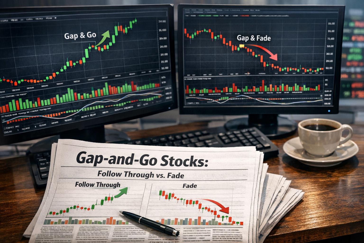
Gap-and-go setups usually try to focus on breakaway and continuation-type gaps—basically the gaps most likely to become “real trading moves” instead of quick chart blips.

Core Principles of the Gap-and-Go Strategy

The gap-and-go strategy rests on a simple behavioral model: a strong directional price shift at the open can create a feedback loop. When the stock opens up (or down) and continues pushing, momentum traders pile in. That demand or supply can broaden the move—at least long enough for day-traders to act.

In most gap-and-go playbooks, execution happens early—often within the first hour after the open. Some traders narrow it further to the first 5 to 30 minutes, when volatility is highest and the market is still deciding whether the gap will become a trend or disappear.

To keep the strategy from turning into “vibes trading,” many practitioners combine a small set of structural conditions:

• A measurable percentage gap relative to the prior close
• Pre-market activity that is meaningfully above average
• A clear catalyst that can justify repricing
• Price holding above (or below) key pre-market reference levels

Traders also watch pre-market highs and lows. These can become the first legitimate “support” or “resistance” once the regular session starts, because the market often treats them as a reference grid.

When Gaps Follow Through

Not every gap gets follow-through. Many gaps reverse quickly, filling part or all of the discontinuity. So traders look for confirmation. Follow-through is more likely when several factors line up.

Strong Catalyst: Earnings surprises, raised or lowered guidance, regulatory approvals, mergers, major sector upgrades/downgrades, or macroeconomic developments can all change valuation. If the catalyst is credible and institutions reposition based on it, the order imbalance can persist beyond the opening auction.

High Relative Volume: Volume matters because it tells you whether the move has participation behind it. Traders often look for volume above typical levels for that stock (and for that time of day). If early-session volume is strong and continues, it suggests broad buy or sell interest rather than a thin-spread “pop.”

Because institutions manage a large portion of market volume, their involvement tends to make continuation more realistic. A gap driven mostly by lightweight flows can peter out fast.

Market Trend Alignment: A gap up during a broadly bullish market environment has a better chance of continuing than a gap up against a risk-off tape. Similarly, a gap down occurring when the broader market is already under pressure may find buyers less willing to step in.

This doesn’t mean “always trade with the trend.” It means that countertrend moves typically face more friction from the crowd.

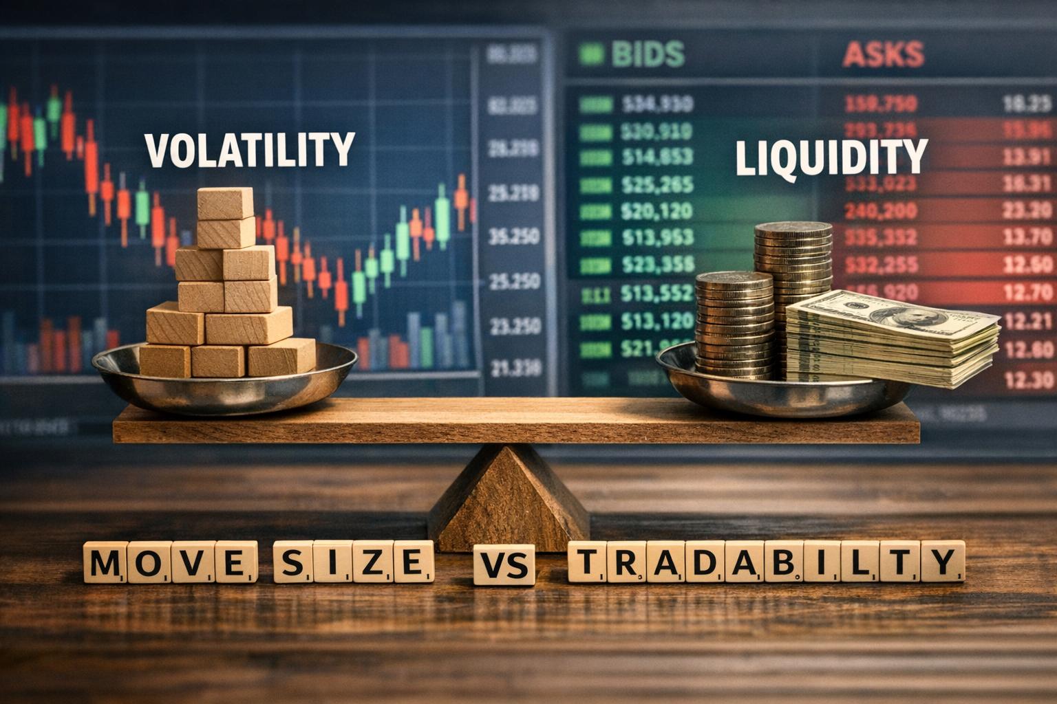
Float and Liquidity Considerations: Stocks with smaller public floats can move more sharply because fewer shares are available to absorb demand. That can help generate a gap-and-go move that “runs.” It also raises the risk that liquidity dries up and price whipsaws.

Larger-cap names are usually more orderly. They can still trend on a gap, but they often require more sustained volume to keep going in a clean way.

Holding Key Levels: One of the most practical tells is how price behaves after the opening push. If the stock opens and then consolidates near the top of the opening range (in a gap up scenario) rather than immediately retracing toward the prior close, it can indicate buyers are absorbing supply. That behavior often precedes another expansion.

Opening Range Dynamics

The opening range—commonly the high and low of the first 5, 15, or 30 minutes—becomes a reference line for many active traders. It effectively captures the market’s earliest consensus about price value before momentum either catches fire or burns out.

– In a gap up, a breakout above the opening range high on strong volume can confirm continuation.
– In a gap down, a breakdown below the opening range low on strong volume can confirm continuation.

False breakouts are common, though. They often happen when volume fades or when the broader market acts differently than expected. That’s why some traders don’t rush the moment price ticks past the opening range high; they wait for consolidation and re-acceptance, which is basically the market saying, “Yeah, we meant it.”

When Gaps Fade

Gap fading happens when price reverses direction and retracts toward the previous session’s closing price. When the price returns all the way to the prior close, traders call it “filling the gap.” (In practice, many partial fades happen too, which can still matter a lot for traders.)

Several conditions make fades more likely:

Lack of Substantive News: If the gap comes from speculation, low-credibility headlines, or broad market noise rather than company-specific developments, early enthusiasm can dissolve quickly. Without a real driver, the stock often migrates back toward a more realistic value.

Extended Technical Conditions: If the stock gaps up after multiple consecutive strong sessions, it may attract profit-taking. Oscillators like the Relative Strength Index (RSI) can contribute to this behavior; if RSI is stretched, traders who bought earlier may lock in gains right when the stock looks impressive again.

Low Early Volume: Volume that never materializes is a yellow flag. A visible gap with thin intraday participation suggests that the move may not have institutional sponsorship. Retail flows alone can move price briefly, but they struggle to sustain an orderly trend.

Higher Timeframe Resistance: If the gap pushes price directly into a major daily or weekly resistance level, selling interest tends to increase. People who bought near that level previously may exit, adding supply right where the stock is trying to go.

Broader Market Reversal: A technically strong setup can still fade if new macro information flips the broader risk environment. When indices change tone, individual stocks often get dragged along, for better or worse.

Many traders treat fading as a separate strategy. They wait for confirmation like a breakdown below early support in a gap up scenario, or rejection below resistance in a gap down case.

Volume Analysis in Depth

Volume is one of the most important variables in gap trading. But “volume” doesn’t just mean the raw number of shares traded; it means how current trading compares to what’s typical.

That’s why traders prefer relative volume: current volume divided by historical average volume for the same time window (or the same trading profile). Relative measures are more meaningful because different stocks have different baseline liquidity.

Common volume observations include:

• Acceleration of volume into breakouts (a sign demand is expanding)
• Volume contraction during consolidations (a sign the move is pausing rather than dying)
• Climactic spikes (sometimes a sign the market is burning through available participants fast)

A continuation move usually requires steady participation throughout the morning. If volume spikes hard at the open and then falls off quickly, the market may have already absorbed the initial imbalance. In that scenario, the stock can drift, retrace, or chop until something else changes.

If you’ve traded gaps before, you’ve probably seen the pattern: it screams for 10 minutes, then suddenly it can’t get momentum back. That’s not always “bad,” but it often means your entry timing needs to be less hopeful and more evidence-based.

Technical Tools and Indicators

Price and volume do most of the talking, but many traders still use additional technical analysis tools to support decisions. The trick is not to let indicators drive the trade blindly. They’re more useful as secondary confirmation—especially when volatility and spreads can make raw price action confusing.

Moving Averages: Intraday moving averages such as 9-period and 20-period exponential moving averages can help identify short-term direction. When price is holding above those averages after a gap up, it suggests bulls have control and dips may get bought. If price continually tags below the short intraday averages, continuation confidence weakens.

On higher timeframes, the 50-day and 200-day moving averages often function as widely watched support/resistance zones. A gap up that runs into the 200-day area, for example, may face heavier selling because lots of traders expect it.

Relative Strength Index (RSI): RSI above 70 or below 30 is often described as overbought/oversold. In strong trends, RSI may stay elevated or depressed longer than you’d expect. For gap-and-go traders, RSI is typically more useful for spotting extremes and potential exhaustion rather than acting as a strict buy/sell signal.

VWAP (Volume Weighted Average Price): VWAP matters because it approximates the average execution price weighted by volume. Many institutional traders treat VWAP as a fairness line. In a gap up day, holding above VWAP can indicate sustained institutional support. Losing VWAP and failing to reclaim it can indicate weakness—particularly if the opening move fails to expand.

In a gap down scenario, trading below VWAP and rejecting attempts to reclaim it can support the bearish continuation thesis.

MACD (Moving Average Convergence Divergence): MACD can add supportive context through crossovers or histogram trends. Since it’s a moving-average-based indicator, it has lag, so it typically won’t tell you the gap move is happening in the first few minutes. It’s better as a supporting view, not a trigger.

Indicators are tools, not fortune tellers. The more you treat them like “weighing factors” alongside price structure and event context, the less you get surprised.

Risk Management Considerations

Gap trading can produce big intraday moves, and that can be fun right up until it isn’t. Volatility increases at the open, spreads can widen, and price can move faster than you can comfortably think. Risk management is what keeps a bad day from turning into a permanent one.

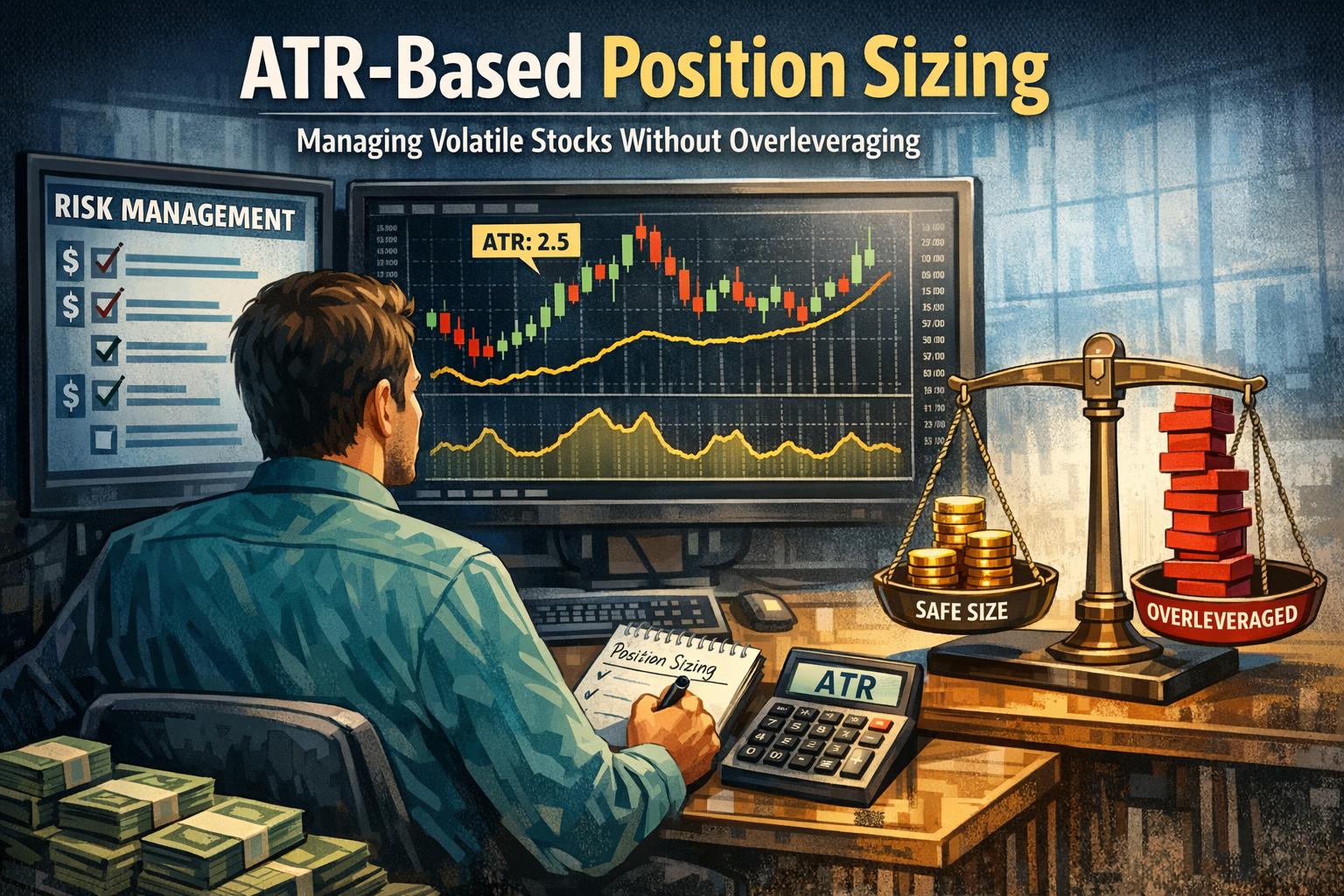
Position sizing: Many traders reduce size during very high-volatility gap days. A smaller position helps keep emotional decision-making from wrecking the trade.

Stops and invalidation levels: Stops vary by style, but common references include pre-market lows/highs, opening range levels, and predefined percentage loss thresholds.

Possible stop placement ideas include:

• Below the pre-market low (for long positions)
• Below the opening range low
• At a fixed percentage loss threshold

The goal isn’t to make the stop “perfect.” It’s to make sure your thesis fails when price does something that contradicts it.

Profit targets: Profit-taking approaches vary with liquidity and volatility. Some traders use prior daily resistance/support as targets. Others use measured moves: for example, projecting a move equal to the initial range expansion. Trailing stops are also used when price trends cleanly after the open.

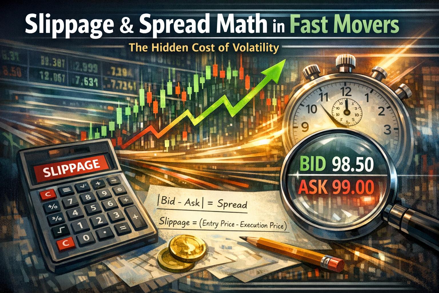
Slippage: Slippage is real in lower-liquidity securities, especially when the bid-ask spread is wide. Your stop might get triggered at a worse price than you expected. That’s one reason some traders prefer higher-liquidity names for gap-and-go—less drama with fills, more predictable execution.

A personal note from real trading life: I’ve watched a stock “barely” break your stop level by pennies and still clip you for a bigger-than-expected loss because spreads widened during the move. That’s not market manipulation—it’s just math. Your risk plan should assume friction exists.

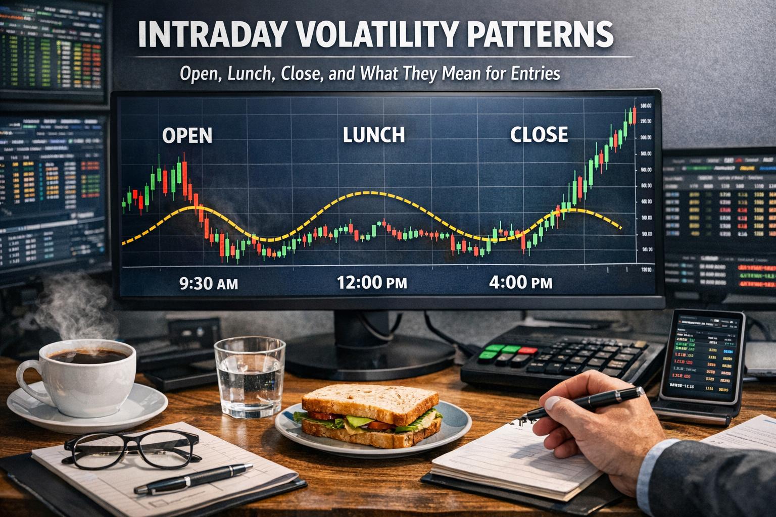
Time-of-Day Effects

Volatility usually peaks near the open and again near the close. The first hour tends to concentrate both order imbalance and decision-making. By contrast, midday trade activity often quiets down: ranges narrow, volume drops, and price becomes more mean-reverting.

For gap-and-go traders, the most actionable window is often the first 30 to 90 minutes. That’s when the market most actively “checks” whether the gap has continuation characteristics. If price shows no directional resolution later in the morning—no consistent pattern of higher highs / higher lows in a gap up, or lower lows / lower highs in a gap down—continuation probability often declines.

That said, markets are unpredictable. A gap that doesn’t trend early can still explode later if new information emerges mid-day (another headline, revised macro expectations, a sudden analyst note) or if the broader market shifts momentum.

So the trade might not follow through at 9:40 a.m., but it might show up at 2:15 p.m. The difference is that “gap-and-go” often implies you’re acting early. If you wait too long without new catalysts, you may be holding a different strategy than you think you are.

Differences Between Large-Cap and Small-Cap Gaps

Not all gaps trade the same. Capitalization level changes liquidity, spread behavior, and how institutions participate.

Large-cap gaps: Large-cap stocks generally have deeper liquidity, tighter spreads, and more stable price increments. Continuation moves may be smaller in percentage terms compared to small caps, but they often still offer meaningful absolute movement. The trading process tends to be cleaner: less random wickiness, easier execution, and more consistent order book behavior.

Small-cap gaps: Small caps can produce larger intraday percentages, especially when float is limited. That sounds great until you remember you’re trading a name where fewer shares exist to absorb demand changes. Small caps often experience wider bid-ask spreads and can face sudden reversals. Halts due to volatility are also more likely in some environments, which is a whole separate type of “fun.”

Institutional participation also differs. Large-cap gaps have a better chance of attracting broad institutional attention, which supports continuation when the move is real. Small caps can still trend, but they may trend on different mechanics—more retail influence, more liquidity swings, and sharper momentum bursts.

In practice: if you’re new to gap-and-go, large caps can be more forgiving. If you can handle the execution risk, small caps can pay—but you’ll need discipline.

Psychological and Behavioral Factors

Gap trading isn’t just math; it’s crowd behavior. A gap-and-go move often draws participants into a storyline: “This should go.” If enough people act on that belief, price tends to follow.

Several behavioral forces come up repeatedly:

Fear of missing out (FOMO): When price opens and quickly moves in one direction, traders who didn’t get in early may chase. That demand/supply can create the momentum traders need to keep the trend going.

Short covering: In a gap up situation, short sellers may be forced to cover. That adds incremental buying pressure, which can accelerate the move. In a gap down scenario, margin calls or risk reductions can intensify selling pressure.

Forced liquidation: Leveraged traders sometimes get squeezed by price movement against their positions. When liquidity is thin, liquidation can become the driver rather than the catalyst.

Short-interest levels and borrow rates can add context—particularly if a gap direction seems consistent with potential covering. Still, don’t treat positioning data like a trigger. Behavioral reactions are probabilistic. You can estimate odds, but you can’t command them.

Data Review and Performance Evaluation

The gap-and-go strategy improves when you review outcomes. If you only trade the days you “feel good about,” you’ll miss the patterns that actually matter—because markets don’t care about your mood.

Systematic traders often keep gap logs across different market cycles. Common metrics include:

• Gap percentage magnitude
• Time to high or low of day
• Percentage of gaps that fill within the same session
• Volume relative to 30-day averages

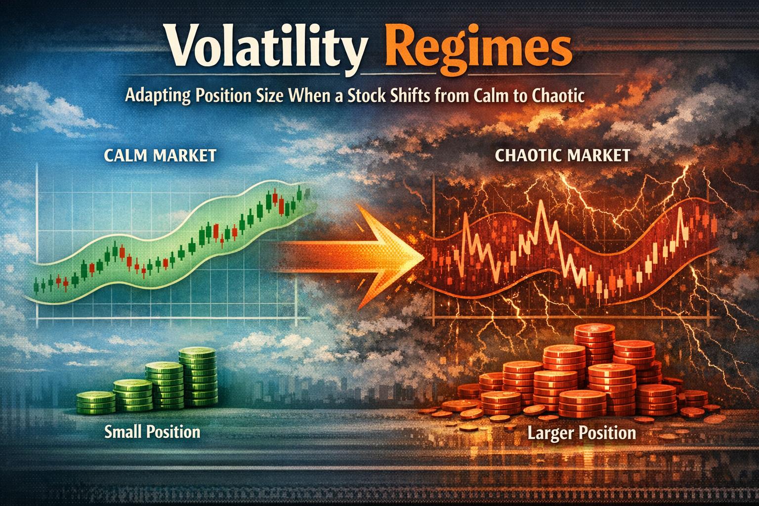
Reviewing historical outcomes under different volatility regimes helps you refine entry criteria. For example, you might notice that continuation is most common after gaps with strong volume and clear catalysts, but reversals spike when gaps happen during broader index pullbacks.

You can also separate results by scenario type: breakaway vs continuation, and gap up vs gap down. The market often behaves differently depending on the direction and on whether the stock is already extended.

At the end of the day, evaluation turns “smart intuition” into a repeatable process. It also exposes the days where you force trades that your own rules told you to avoid. Those days tend to stand out in your P&L for the wrong reasons.

Common Gap-and-Go Mistakes

Even careful traders make predictable errors. It’s useful to know what these usually are:

Trading the gap without verifying participation: A gap can look dramatic, but if relative volume is weak, you’re trading a story without witnesses.

Ignoring the broader tape: If the index is reversing hard, individual continuation moves can lose their footing. You don’t need to demand perfect correlation—just don’t ignore obvious conflict.

Entering too late after a fading attempt: Some traders wait for confirmation and accidentally buy after the move has already failed. Confirmation matters, but so does “where in the day” and “how price is behaving now.”

Using stops that don’t match the thesis: A stop based on a random percentage can be wrong for a specific setup. Better stops align with structural invalidation, like pre-market breaks or opening range failures.

Overtrading: Gap days can create multiple signals in a single name, and momentum traders sometimes feel compelled to act on every shift. Overtrading usually means more small losses that pile up—like crumbs you’ll trip over later.

Mistakes aren’t always fatal. But the ones that show up repeatedly are usually fixable, which is the good news.

Putting It All Together: A Practical Checklist

A gap-and-go trade usually becomes sensible when the conditions match up quickly. Here’s how many traders conceptualize it, without pretending there’s a magic formula hidden in the chart.

First, confirm the gap is a meaningful repricing event. Look for a catalyst that explains the move and check whether the stock has the liquidity profile to support intraday continuation.

Second, verify participation. Is pre-market activity stronger than usual? Does early regular-session volume show up quickly and hold near breakout attempts rather than disappearing?

Third, watch price structure after the open. Does price hold key reference levels such as pre-market highs/lows or VWAP (when you use it)? Does it respect the opening range, or does it immediately retrace?

Fourth, align the setup with broader market conditions. You don’t need the index to be bullish in every gap up trade, but it shouldn’t be actively fighting your direction.

Finally, execute with a stop that invalidates your thesis and use profit logic that fits the day’s volatility. If you’re trading a fast mover, waiting for a perfect target can turn a clean trade into a messy one.

Conclusion

The gap-and-go strategy focuses on price discontinuities at the start of the trading session, then tries to profit from continuation in the same direction. A gap is the market’s initial repricing event—but continuation depends on whether there’s enough fuel behind it.

Gaps tend to follow through when catalysts are credible, relative volume supports the move, market direction aligns, key structural levels hold, and liquidity allows price to trend instead of just spiking. When participation is weak or the catalyst isn’t substantive, gaps more often retrace toward the prior close and fade back into yesterday’s price.

In practice, differentiating continuation from fade requires combining price action, volume analysis, technical references like the opening range and VWAP, and awareness of broader market conditions. And just as importantly, gap-and-go trading depends on risk management: position sizing, realistic stops, accounting for slippage, and consistent review of results.

When approached systematically rather than impulsively, gap trading can operate as a defined intraday methodology inside a broader trading framework.

Understanding Intraday Volatility Patterns

Intraday volatility is the magnitude and pace of price movement inside a single trading day. It’s not just “markets being random” (though they sometimes act like it). Instead, the way volatility shows up across hours tends to repeat with enough consistency that experienced traders plan around it.

At a basic level, volatility measures how quickly prices change. In practice, intraday volatility matters because it affects transaction costs, execution quality, stop-loss placement, and the odds that a strategy behaves the way you think it will. If you’ve ever wondered why a setup that works great at the open falls apart at lunch—or why the close suddenly feels like the last episode of a show everyone binges—you’re already seeing the same mechanism.

Volatility itself reflects the rate at which prices change, and it’s influenced by order flow, liquidity, macroeconomic releases, institutional participation, and behavioral factors. Daily and longer-term volatility get a lot of attention, but intraday volatility is especially relevant for short-term traders, algorithmic systems, and execution desks that care about minimizing slippage and improving fills.

The typical intraday shape: why volatility isn’t evenly spread

Many equity markets show a “U-shaped” volatility profile: higher volatility near the open, lower movement during midday, and a re-acceleration near the close. That pattern shows up often enough to build intuition, but it’s not a law of physics. Variations appear across asset classes, market regimes, and news schedules.

To make it useful, you need to understand what’s driving each part of the session:

• Liquidity (how easily you can trade without moving the price)
• Order flow (how much buy vs sell pressure hits the market)
• Information flow (what new data is arriving and when)
• Execution needs (when institutions must trade)
• Microstructure effects (bid-ask spreads, market depth, auctions)

When those ingredients change across the day, volatility changes with them.

The structure of the trading day (and why it matters)

Most liquid markets—even if they don’t all have exactly the same hours—can be mentally divided into three broad phases:

• Opening phase
• Midday phase
• Closing phase

Each phase tends to have a different mix of liquidity and order flow. That matters because the same percentage move can mean different trading conditions depending on time. For example, a 0.5% move on a thin midday tape typically results in worse execution than a similar move that happens during open auction conditions—at least for many retail participants and smaller desks.

Understanding how volume and volatility interact during these segments helps with practical decisions such as:

• Trade timing
• Position sizing
• Stop-loss placement
• Profit targets
• Order execution methods

Importantly, the dynamics of these phases aren’t only about charts. Human behavior shows up too. Institutions tend to cluster activity around known execution windows, while retail traders often become more active around the open or after headline-driven events.

The open: market opening volatility

The first portion of the trading day—especially the first hour—typically shows elevated volatility and higher volume. This is where the market absorbs the overnight information that built up while exchanges were closed. It’s the “read the news, now place the bets” portion of the day.

Common drivers include:

• Corporate earnings announcements
• Macroeconomic data releases
• Geopolitical developments
• Overseas market movements
• After-hours trading activity

Because overnight information continues to evolve while the exchange is shut, the open becomes the main time for price discovery. That price discovery process is quick and messy. It usually shows up as wider bid-ask spreads, sharp swings early on, and sometimes strong directional moves in certain names.

Price discovery and order imbalance

In many markets, the open involves an auction mechanism. Orders submitted before the official session open get aggregated, and the opening price forms based on the balance between buy and sell demand—plus market rules around execution.

When there’s meaningful order imbalance, you get opening gaps. A stock can open significantly above or below its prior close after major announcements, simply because the market reprices the asset before it can trade continuously.

In this situation, opening volatility often reflects:

• Rapid reassessment of fair value
• Concentrated “first prints” as the market starts trading
• Execution urgency from participants who missed prior trading hours

If you’ve ever placed an order right at the bell and watched the price move away before your fill—welcome to opening volatility. The open can reward speed and penalize impatience.

The opening range concept

Many traders use the opening range as an anchor. It typically refers to the high and low established in the first 5 to 30 minutes. The logic is straightforward: if enough participants agree on direction early, the range often becomes a battleground.

A break above the opening range high with convincing volume is often interpreted as upward momentum. A break below the range low can be interpreted as downside intent.

However, false breakouts are common. The open is where positioning changes hands quickly, and the market often “tests” levels before committing. So while traders use the concept as a reference, confirmation tends to matter more than the line itself.

In practice, traders often combine opening range logic with:

• Volume and trade counts
• Order book depth or liquidity measures
• Momentum indicators (but not blindly)
• VWAP or VWAP deviations to judge mean pressure

A breakout that happens on thin volume is more likely to fade than one where aggressive buying (or selling) overwhelms the opposing side.

Risk considerations at the open

Even if the open offers opportunities, it also brings hazards. The main risks are costs and execution quality.

• Wider spreads raise transaction costs, especially for limit orders that sit near the wrong side of the book.
• Rapid reversals increase slippage and stop-outs.
• Market orders can execute at unfavorable prices because price can move while your order is working.
• Volatility may decline fast after an initial spike, meaning early entries can turn into red positions if you misjudge timing.

This is one reason you’ll see two fairly different behavior patterns among traders:

• Some wait for stabilization, then enter with a calmer read on direction.
• Others trade the first burst itself, using tight risk controls and expecting fast movement.

Both can work. Just don’t mix their rules by accident. If you plan to scalp, don’t size like you’re investing. If you plan to invest, don’t treat the open like a casino roulette wheel.

Lunchtime: a midday lull

After the initial opening volatility cools off, markets often enter a lower-activity period—late morning into early afternoon in many equity sessions. This is the midday lull where the chart looks flatter, but “flatter” doesn’t always mean “safe.” It often means fewer participants are actively pushing price.

Typical features include:

• Lower trading volume
• Reduced price ranges
• Slower order flow
• Less follow-through when breakouts first appear

Several factors contribute to this pattern:

• Major economic data releases typically occur earlier in the day.
• Institutional desks may slow down temporarily while workflows shift.
• Retail participation can drop during work hours.
• Some algorithms shift toward passive liquidity provision rather than aggressive trade-taking.

As participation declines, liquidity can become thinner. Thin liquidity can compress movement when nothing happens… but when something does happen (a stop cascade, a headline, a large order), the move can happen quickly. So midday is often “quiet until it isn’t.”

Consolidation and range trading behavior

Midday markets frequently consolidate. Prices drift sideways inside support and resistance zones. Breakouts can occur, but follow-through may be weak because fewer buyers and sellers are actively willing to continue the move.

That makes midday conditions attractive for range traders. In this environment, mean and reversion behavior tends to show up more than trend persistence.

Range traders may:

• Buy near support levels
• Sell near resistance levels
• Use smaller profit targets
• Maintain tighter stop-loss levels

Trend-following strategies can struggle here if volatility drops sharply. A trend needs fuel—often provided by persistent order flow. Midday often provides less of it, which can cause trend systems to churn.

One practical note: “works in backtests” during midday can still fail in live trading if execution quality is poor. Liquidity matters. Even a great signal can underperform if fills are inconsistent.

Liquidity considerations during low participation

Reduced volume affects execution. A large order placed during this window may influence price more than expected relative to average market depth.

Institutional participants often avoid initiating substantial positions during low-liquidity periods unless there’s a strategic reason—such as portfolio rebalancing, mandated trades, or scheduled hedging.

Meanwhile, many algorithmic strategies reduce participation rates midday to reduce market impact. They might still trade, but they behave more like a gentle breeze than a bulldozer.

To a trader, this shows up in:

• Wider micro bid-ask spreads relative to the day’s midday averages
• More frequent “stalling” near levels
• Lower volatility but sometimes sudden spikes around specific events

So midday can be good for patience and poor for forcing trades.

The close: increased activity near market close

Volatility often rises again in the final hour of trading. This closing period tends to involve adjustments and “finish work” activity. Traders often want to set exposure before the session ends, especially for assets where closing prices matter for benchmark calculations.

Closing volatility is influenced by:

• Portfolio rebalancing
• Index fund adjustments
• Options hedging activity
• Intraday trader position unwinding
• Execution of market-on-close orders

Many markets use a closing auction similar in concept to the opening auction. Orders accumulate, then execute at or around the close price. When large order flow arrives near the end, price can shift quickly and momentum can briefly dominate.

Institutional participation and benchmark mechanics

Institutions often prefer executing near the close to reduce tracking error versus benchmark indices. Benchmarks can be calculated using closing prices, which makes the close a practical anchor point for many portfolio managers.

When institutional participation increases, trading volume often rises. It can also bring sharp price changes—particularly if program trading, index reconstitution, or hedging pressure hits at the same time.

If you observe rising order flow, volume acceleration, or a momentum shift late in the day, it’s usually wise to:

• Tighten risk controls
• Be cautious about assuming the midday regime will persist
• Consider whether your intended hold time extends beyond the close

Late-day trading can feel like the market is “locking in.” That’s because it is, in a way.

End-of-day strategies: what traders actually do

Traders often develop tactics specifically for the last part of the session. Common approaches include:

• Trend continuation trades when the day’s direction remains intact.
• Mean reversion trades when price deviates significantly from intraday averages.
• Overnight positioning when traders expect continuation into the next session.

Overnight positioning adds another layer: after-hours news can hit, and gaps can form at the next open. So decisions made near the close often include explicit assessments of overnight risk, such as upcoming economic releases or earnings.

Practical example: suppose a stock rallies strongly into the last 30 minutes after a favorable macro report. A trend continuation trader might hold for a planned overnight move. But a mean reversion trader might expect buyers to fade once the “need to buy now” pressure (index-related, hedging, or end-of-day forced execution) passes.

Both can be rational. The difference is the model each trader uses for order flow and price behavior—and how well it matches what’s actually happening.

The U-shaped volatility curve (and why it keeps showing up)

If you plot intraday volatility across time, it often forms a U-shape: high at the open, lower around midday, and higher again near the close. This pattern has been observed across decades in equity markets and appears consistently enough that it’s become part of standard market intuition.

Empirical research supports the idea that intraday trading activity and liquidity distribution help produce persistent volatility structure. But there are plenty of exceptions.

• Central bank announcements can elevate midday volatility.
• Earnings releases during trading hours can disrupt the normal intraday pattern.
• Geopolitical developments can create sustained volatility across multiple periods, not just the open and close.
• Market regime changes (risk-off periods, high headline sensitivity) can increase baseline intraday volatility.

So yes: the U-shape is useful. But the market has a habit of changing its mind when new information arrives. Real-time context still matters.

Role of algorithmic trading and high-frequency trading

Modern markets run on algorithms, and that includes strategies that directly influence liquidity and price movement. These systems react to order imbalances, spreads, and statistical signals within milliseconds (and for many assets, that’s plenty fast to matter).

Algorithmic trading can both dampen and amplify intraday volatility:

• Market-making algorithms may stabilize prices by supplying liquidity and narrowing spreads.
• Momentum algorithms may accelerate directional moves when signals confirm or when order flow trends.
• Statistical arbitrage systems may compress spreads across correlated assets, reducing volatility in relative terms but sometimes increasing volatility during brief dislocations.

The concentration of algorithmic participation around opening and closing auctions can intensify those intervals. Algorithms often treat those auctions as predictable high-activity environments—so their collective behavior can create bursts of volatility.

That’s also why you can’t judge volatility only from your chart’s candle size. Microstructure effects matter. A period that looks calm visually might still involve fleeting liquidity gaps that affect execution quality.

Implications for trade entries (time-of-day isn’t cosmetic)

If intraday volatility changes across the day, then entry timing affects probability distribution of outcomes. A “good” signal might still underperform if you enter at a time when the market’s variance and liquidity conditions are fundamentally different.

During the open: what to expect

Traders active early should prepare for quick movement and fast regime shifts.

• Assume rapid price movement and plan for it.
• Use predefined stop-loss levels rather than improvising mid-chaos.
• Account for slippage and spread impact.
• Evaluate pre-market data and news, not just the first candle.

Breakout and momentum strategies often appear during this window. Still, position sizing tends to need more attention because the volatility distribution at the open differs from midday.

A common mistake: entering with the same size as midday because the setup “looks the same.” It might not be. The candle is not the strategy; the market conditions are.

During midday: trade selection matters more

During the lunch lull, traders often need to adjust how they think about signals. Lower volatility can reduce range opportunities, but it can also make mean reversion more workable.

• Scale back position size to reflect thinner liquidity.
• Favor mean-reversion setups if the market consolidates.
• Use technical analysis for structure, not for prophecy.
• Avoid initiating trades without clear volume confirmation.

Midday execution can also be trickier because fewer active traders can mean your order interacts with the market differently than it would in higher-volume windows.

So if you’re trading midday, consider whether your expected edge depends on continuous order flow or whether it survives intermittent liquidity.

Near the close: watch for auction effects

As the close approaches, you’ll often see volume acceleration and short-term trend behavior. That doesn’t mean every stock trends. It means the market shifts toward execution-driven flow.

• Monitor volume acceleration and order flow changes.
• Adjust trades to align with intraday direction.
• Reduce exposure if you want less overnight risk.
• Anticipate volatility spikes linked to auction mechanisms.

Effective trade management near the close frequently depends on order types and auction mechanics such as market-on-close or limit-on-close orders. Using the wrong order strategy at the wrong time can make “right idea, wrong execution” happen in real life.

Risk management across intraday phases

Risk management isn’t only about your stop-loss price. Intraday volatility affects leverage, risk-reward ratios, and how often stops get hit by noise.

The practical move is to treat time-of-day as part of risk modeling.

Key considerations include:

• Adjusting stops to reflect time-of-day volatility averages.
• Avoiding overtrading during low-volatility intervals that don’t offer enough reward for churn.
• Reducing leverage during high-volatility announcements to avoid blowups from short-term spikes.
• Monitoring cumulative daily risk exposure rather than thinking each trade is isolated.

Some traders use average true range (ATR) calculated over intraday time frames to adjust expectations. ATR isn’t magic, but it’s a pragmatic way to translate volatility into more realistic stop distances and target ranges.

A simple mental model helps: if ATR is higher near the open, then the market naturally produces wider “normal” swings. Your stops can’t assume midday behavior while trading open conditions.

Application across asset classes

The U-shaped pattern shows up most clearly in equity markets, especially those with auction mechanisms. Still, the idea that volatility clusters by time holds across other asset classes too—but with different drivers.

Futures markets

Futures can show strong reactions to economic releases and can trade more continuously than many equity sessions. That means volatility spikes can occur around events that may not align neatly with equity open or midday.

You might see volatility rise around:

• Scheduled macroeconomic announcements
• Major commodity supply updates
• Geopolitical risk headlines affecting risk sentiment

Even when midday looks calm, futures can remain jumpy if news timing hits during those hours.

Foreign exchange (FX)

FX markets operate continuously throughout weekdays. Intraday volatility typically clusters around regional session overlaps. For many participants, the London–New York overlap often brings elevated activity because liquidity and participant overlap increase.

So instead of “open and close” in the equity sense, FX traders think in terms of:

• Tokyo session activity
• London session liquidity
• New York overlap and closing adjustments

This matters because a strategy designed for a quiet time in equities might land right in the middle of an FX overlap window.

Cryptocurrency markets

Cryptocurrency markets trade 24/7 and lack a centralized closing auction comparable to equities. So the traditional U-shape won’t map perfectly.

Still, liquidity and volatility can increase during times aligned with major financial centers. When Bitcoin and major alts experience liquidity shifts, it often mirrors broader participant activity. So while the mechanism differs, time-based volatility clustering can still show up.

Also, crypto has its own behavior quirks: leverage, liquidations, and reflexive order book effects can create sharp volatility spikes that aren’t always “orderly” in the way many equity sessions are.

Data analysis and measurement of intraday volatility

To work with intraday volatility patterns, you need measurement tools and a method for validating whether a pattern holds for your specific market, timeframe, and strategy.

Common analytical approaches include:

• Standard deviation of returns over intraday intervals
• Volatility heat maps
• Volume-weighted average price (VWAP) deviation analysis
• Intraday range statistics (high-low ranges by time bucket)
• Order flow imbalance metrics

A frequent workflow looks like this:

• Segment the trading day into time buckets (for example, 5-minute or 15-minute intervals).
• Compute volatility metrics per bucket for historical data.
• Average the results across multiple days to estimate typical behavior.
• Compare the averages to the current regime and event schedule.
• Test whether your strategy edge still holds after spreads, slippage, and real execution constraints.

This approach makes the volatility pattern practical. It turns “seasonal” intraday intuition into a quantifiable assumption you can stress-test.

One caution: intraday data quality matters. If your data feed handles late prints differently or your historical candles don’t reflect the same market microstructure, your measurements can drift. That’s the kind of bug that politely wastes months of your life.

Putting it all together: practical ways traders use intraday volatility patterns

Many traders don’t “trade the model.” They use volatility patterns to make better decisions about execution and risk.

Here are a few realistic examples of how this looks in day-to-day trading:

Example 1: Stop placement depends on where you entered

If you place stops without considering the time-of-day volatility regime, you’ll often see stop-outs cluster at particular times. For example, a stop distance that fits midday noise might be tight during open conditions. Adjusting stop distance using intraday volatility averages can reduce random churn.

Example 2: A midday mean reversion setup might be a lunchtime trap

Midday can favor range trading, but only when liquidity behaves as expected. If a midday period overlaps with an unexpected news catalyst, volatility may not compress as usual. A trader following “midday always ranges” thinking can end up trading against a new regime.

Example 3: Close strategies need auction-aware execution

Closing volatility often comes from execution-driven order flow. Traders who ignore auction mechanics might find their orders don’t fill where they expected. Using the right order type and considering market-on-close behavior can matter more than the indicator signal.

Conclusion

Intraday volatility patterns give you a structurally informed way to understand how markets behave across the trading day. Higher activity around the open reflects price discovery and rapid incorporation of new information. Reduced movement in the midday hours often aligns with lower liquidity and more consolidation behavior. Volatility tends to pick up again near the close due to institutional participation, portfolio adjustments, options hedging, and auction-driven execution mechanics.

Recognizing these recurring dynamics helps traders refine entry timing, adjust stop placement, and align strategy behavior with the market conditions that actually exist at each hour. That said, intraday patterns aren’t immune to regime shifts. Central bank announcements, earnings surprises, and geopolitical shocks can change the usual profile quickly.

So the goal isn’t to memorize the U-shape and call it a day. It’s to treat time-of-day volatility as a real input—then keep your eyes open when the market decides to do something else. Continuous analysis and disciplined execution remain the boring, effective part of trading. And yes, boring is sometimes the best flavor.

Understanding Volatility and Liquidity in Financial Markets

In financial markets, two terms come up in pretty much every serious conversation: volatility and liquidity. People throw them together because they often move in the same general direction during stress, but they describe different realities. Volatility is about how much prices move. Liquidity is about how easily you can trade without pushing the price around. If you mix those up, you end up with a risk model that looks good on paper and behaves badly in the real world.

For investors and traders, getting the distinction right matters because it touches three practical areas: price formation, trade execution, and risk management. And it comes up across asset classes—equities, bonds, commodities, and currencies—though the details vary a bit depending on how those markets operate.

Defining Volatility

Volatility refers to the degree of variation in the price of a financial instrument over a defined period. In plain English: it measures how “jumpy” the price is. When volatility is high, the instrument tends to experience wider swings—sometimes minute to minute, sometimes day to day. When volatility is low, prices drift within narrower ranges.

Most volatility measures are variations of the same idea: dispersion. In practice, you’ll see volatility defined as:

• Standard deviation of returns (common in risk models)
• Variance (same concept, just another mathematical form)
• Average true range (often used in technical analysis to gauge typical movement)

High volatility doesn’t only mean “higher risk” as a slogan. It also affects how traders behave. Wider price swings attract momentum strategies, increase the frequency of stop-outs, and change hedging costs. If you’re trading options, volatility is basically the weather system that governs the entire pricing model.

What drives volatility?

Volatility spikes for reasons that tend to be common across markets:
Corporate earnings and guidance changes
Macroeconomic data releases (inflation, jobs reports, central bank signaling)
Geopolitical events and policy shocks
Shifts in market expectations—sometimes subtle, sometimes not

A useful way to think about it is this: volatility rises when new information arrives faster than markets can comfortably price it. That can happen during scheduled events (like rate decisions) or unexpected ones (like a sudden regulatory change).

Historical vs. implied volatility

Volatility is often measured using two broad approaches:

• Historical volatility: calculated from past price data. It answers, “How much has it moved recently?”
• Implied volatility: derived from options pricing. It answers, “How much movement is the market expecting going forward?”

Historical volatility is backward-looking and depends on the chosen window length. A 20-day measure might tell a different story than a 60-day measure, especially if volatility regimes change. Implied volatility is forward-looking in the sense that it reflects option market expectations. That said, implied volatility can represent the cost of hedging or speculative pricing more than a clean forecast. Markets rarely agree on what “will happen,” only on what is being priced.

Understanding Liquidity

Liquidity describes how easily an asset can be bought or sold without causing a substantial change in its market price. A liquid market gives you a smoother execution experience: you can trade larger size, at tighter spreads, with less slippage.

In practice, liquidity shows up through several observable features:

• Tight bid-ask spreads: the difference between what buyers pay and sellers ask
• Deep order books: enough orders on both sides at multiple price levels
• Consistent trading volume: stable participation, not just one-off trades

If those conditions hold, an order can be filled with less “price movement caused by your own presence.” If they don’t, liquidity is thinner. Your trades start to move the market, sometimes dramatically for illiquid instruments and in certain hours.

What affects liquidity?

Liquidity doesn’t exist in a vacuum. It depends on:

• Number of active market participants (more participants often means better price support)
• Trading infrastructure and market structure (e.g., centralized exchanges vs. fragmented trading)
• Regulatory environment (rules can affect participation and market-making)
• Overall market conditions (risk-on vs risk-off changes behavior fast)

Institutional investors tend to care about liquidity more intensely than retail traders because their orders are large relative to typical trading volume. Large orders need depth. Without it, the transaction doesn’t just fill—it “walks” the price. That turns a planned trade into a different trade than expected.

Primary vs. secondary market behavior

One more nuance that’s easy to forget: liquidity can behave differently in primary markets (new issuance) compared to secondary markets (trading after issuance). A bond issued today might not trade particularly well later if dealer inventory risk changes or if there’s little demand for that maturity. It’s not always about the asset’s long-term quality; it’s often about who happens to be holding inventory and how eager they are to adjust it.

Volatility Isn’t Tradability

Here’s a misunderstanding that shows up all the time: high volatility automatically equals a great trading opportunity. It’s a tempting thought because big price moves feel profitable. But volatility is not the same thing as tradeability.

You can have an asset that moves a lot but is annoying to trade. In that case:

• Bid-ask spreads may be wide
• Order book depth may be thin
• Slippage can eat your edge
• Stops might trigger from noise rather than a real breakdown

On the flip side, an asset can be stable (low volatility) and still be a pleasant instrument to trade—especially if it’s liquid and spreads are tight.

Put differently: volatility speaks to price behavior. Liquidity speaks to execution friction. A strategy needs both the right kind of price movement and a market structure that lets you capture it without paying too much in the form of transaction costs and adverse selection.

Real-world example

Imagine two stocks:
Stock A has occasional 5–8% swings intraday, but the spreads widen when news hits and volume thins out between headlines.
Stock B moves more calmly—say 1–2% swings—but it trades steadily with tight spreads and strong depth.

If you’re running a short-horizon strategy that depends on expected execution quality, Stock A might be “tempting on paper.” In reality, your fills may be worse than you assume, and your effective risk/reward can shrink fast after you account for costs. Stock B can outperform simply because trading it behaves like trading should: consistent and measurable.

Interaction Between Volatility and Liquidity

Volatility and liquidity interact in a way that often makes intuitive sense. When markets calm down, uncertainty falls and participation improves. When fear rises, participants demand more compensation for taking risk and trade less freely.

During market stress, you commonly see:

• Volatility rising as returns widen
• Liquidity contracting as bid-ask spreads widen
• Order books becoming thinner because market-makers reduce inventory exposure

This relationship isn’t always one-directional, but it’s frequent enough that traders plan for it. Liquidity doesn’t just disappear randomly; it tends to evaporate when people stop wanting to hold risk.

In calmer periods, liquidity often improves and price changes become more measured. Order books refill, spreads narrow, and trading costs drop. The market feels “cleaner,” and many strategies recover their expected performance because execution becomes closer to theoretical assumptions.

How this shows up in prices

When liquidity decreases and volatility increases at the same time, the price can do something uncomfortable: it can move in larger steps. That can be visible as larger gaps between trades, less orderly progression through price levels, and higher probability of overshooting your intended fill.

There’s also a secondary effect: when liquidity thins, it becomes harder to arbitrage mispricings quickly. That can make volatility persist longer than expected, especially when participants disagree and trading slows down.

Implications for Risk Management

If you only track volatility, you may still get blindsided by the execution and loss mechanics that come from low liquidity. If you only track liquidity, you can still take unmanaged risk during price shock events.

Recognizing the distinctions and interaction between volatility and liquidity helps you do several practical things better:

• Position sizing: scale size not just to volatility, but to the liquidity you can actually trade
• Execution planning: choose order types and timing consistent with market depth and spreads
• Stop and limit logic: avoid assuming you’ll get the fill you want under stress
• Risk controls: include transaction costs and market impact in the “real” loss estimate

A lot of “risk” in trading is not strictly about price direction. It’s about the path you take to get in and out, and whether that path stays close to what your backtest assumes.

Volatility and Liquidity Across Asset Classes

The core concepts apply everywhere, but the expression differs.

Equities

In equities, liquidity often relates to:
Listing venue and market microstructure
Average daily volume
Presence of market makers or active investors
Bid-ask behavior around news

Volatility tends to rise around earnings, macro events, and large system-wide shocks. In highly liquid indexes, volatility might not look extreme relative to the index. Still, individual stocks can have sharp volatility changes because their order flow is more concentrated around specific events.

Bonds

Bonds can be less liquid in practice, even when they appear “major.” Many bond markets rely more heavily on dealer inventory and can have wider spreads, thinner depth, and more uneven pricing across maturities. You might see volatility shift in yield changes and spread widening, while liquidity varies significantly by tenor, credit quality, and issuance size.

A bond can stay relatively stable in terms of headline moves but still be tricky to trade if depth fades when you need it most.

Commodities

Commodity markets include variables like storage costs, futures contract roll dynamics, and supply shocks. Liquidity can differ across contract months. Volatility can spike based on weather, geopolitics, or production disruptions, and trading conditions may worsen when speculative participation drops or hedgers adjust quickly.

If you’ve ever watched a futures curve flinch, you know volatility isn’t just about the front contract. It can ripple through the curve as expectations shift.

Currencies

In FX, liquidity is generally high for major pairs, but conditions still change during specific sessions and events. Spreads can widen during certain liquidity troughs (often tied to time-of-day and regional trading patterns), and volatility can jump around central bank decisions.

Currency volatility can be influenced by changes in interest rate expectations, risk sentiment, and sudden flows. Liquidity can be influenced by who’s active at that time and how risk appetite behaves.

Measuring Volatility and Liquidity in Practice

Most people understand volatility conceptually, but measurement approaches often vary. The same goes for liquidity.

Common volatility measures

Typical tools include:
Standard deviation of returns (for modeling and risk metrics)
Rolling-window volatility (to see regime changes)
Implied volatility from options (for expectation and hedging costs)
Average True Range (ATR) in technical frameworks

It’s worth being a little careful with windows and scaling. A 30-day volatility estimate can lag a regime shift. A 5-day measure might react quickly but be noisy. Many traders and risk managers use multiple horizons.

Common liquidity measures

Liquidity metrics vary depending on whether you want something that’s operational (for execution) or analytical (for risk models). Common ideas include:

• Bid-ask spread (average and distribution)
• Trading volume and turnover
• Order book depth at multiple levels
• Market impact estimates (how price moves in response to trade size)
• Time-to-fill and fill rate (especially for limit orders)

The subtle point: some liquidity measures are static averages; others are conditional. Spreads might average narrow but blow out around events. Depth might look fine most days but disappear at specific times. Good measurement tries to capture the situations where you actually trade.

Execution Costs: Where Liquidity Meets Your Profit Model

Whenever someone says “volatility is high, so returns should be high,” I gently remind them about execution costs. Volatility doesn’t pay you automatically. You pay the market to enter and exit, and you pay for the difference between your intended and actual fill.

Execution costs come from:
Bid-ask spreads
Slippage (difference from expected price)
Market impact (price movement caused by your order)
Adverse selection (trading against better-informed participants)

Liquidity affects all of the above. When liquidity falls, spreads widen and market impact rises. This can make a strategy that looks profitable on paper turn unprofitable in live trading.

A simple way to frame it

If you trade a liquid asset, your expected execution price might be close to the mid-price plus a small adjustment. If you trade an illiquid asset, your execution price can drift far from mid, especially for larger sizes or urgent orders.

This is why sophisticated traders talk about “implementation shortfall.” It’s basically: how much performance you lose between decision and execution.

Volatility Regimes and Liquidity Regimes

Markets don’t stay in one mood indefinitely. Volatility changes over time in regimes. The same is true for liquidity.

A “regime” can mean:
A sustained period where volatility is higher than usual
A market stress period where liquidity systematically contracts
An earnings season window with predictable event clusters

When regimes shift, simple models built on historical averages can break down. That’s why risk managers consider stress scenarios rather than only routine conditions.

Common stress pattern

The typical stress pattern is “more volatility + less liquidity.” It’s inconvenient because many portfolios depend on being able to hedge or rebalance. If hedging instruments become illiquid at the same time volatility rises, you can’t respond quickly enough, and losses compound.

This is one reason liquidity risk deserves its own attention rather than being treated as a footnote after volatility.

Portfolio Construction: Using Both Metrics Without Overcomplicating It

You don’t need a PhD in market microstructure to benefit from the volatility/liquidity distinction. You do need to avoid the habit of treating them as interchangeable.

Position sizing that respects liquidity

Even if your risk model says you can hold a large position based on volatility alone, liquidity may force smaller size in practice. A useful rule of thumb is to estimate whether your order size would consume a meaningful portion of available depth—especially during the times you trade.

If your trade repeatedly pushes against the book, your actual risk becomes larger than expected.

Correlation and risk interactions

Volatility and liquidity also affect correlations. In stress, correlated moves often become more intense. Meanwhile, liquidity constraints can prevent trades that would normally reduce risk through diversification or hedging. That changes the risk profile even if your “static” correlations look reasonable.

So yes, correlation matters. But when correlation rises while liquidity falls, the stress can be extra ugly.

Rebalancing behavior

Rebalancing helps control risk, but only if you can do it cheaply and on schedule. Liquidity influences the feasibility of rebalancing. If spreads widen and spreads widen right when you need to trade, your rebalancing becomes “selective,” and the intended risk reduction may not happen.

Institutional portfolios that rely on scheduled rebalancing often incorporate liquidity forecasts or use trading windows to reduce cost. Retail traders do this less formally, but the pain is similar.

Common Scenarios Where People Get It Wrong

It’s useful to list the failure modes that show up repeatedly.

Confusing “price movement” with “trade execution”

Someone identifies a high-volatility asset and assumes it’s easy to trade that volatility. Then they discover the spreads are wide when the moves happen most. The result: profits get eaten by costs during the exact moments the strategy expects to do well.

Assuming liquidity today equals liquidity tomorrow

Liquidity is conditional. Event-driven markets can change their structure quickly. A market can be liquid most days and temporarily become hostile when volatility rises. If your strategy doesn’t account for that conditional shift, you end up trading blind.

Ignoring the size problem

Small trades can look fine in illiquid instruments. Large trades reveal the truth. Many traders learn (usually the expensive way) that order size relative to depth matters more than average volume.

Practical Tips for Better Decision-Making

Below are practical methods traders and investors use to separate volatility and liquidity thinking, without making it an academic exercise.

Check volatility and liquidity around the events you actually care about

If you trade around earnings, look at volatility and spreads in those windows. Don’t only check average conditions. Execution quality during event windows can differ a lot from “normal days.”

Use liquidity-adjusted assumptions in backtests

Backtests often assume you can trade at predictable prices. That’s fine for textbooks and less fine for real markets. Incorporate realistic spreads and slippage estimates, and adjust them for liquidity conditions.

If you backtest a strategy with constant friction, you may underestimate losses in high-volatility periods.

Stress-test both the price path and the ability to exit

A portfolio can lose money because prices go down. It can also lose money because you can’t exit cheaply. Liquidity stress needs to be part of the simulation.

In other words: stress the exit, not only the entry.

FAQ: Quick Clarifications

Is volatility the same as risk?

Volatility often correlates with risk, but it’s not identical. Risk includes the consequences of not just price movement, but also execution, liquidity, leverage, and position size relative to market depth. Two assets with the same volatility can behave very differently when you try to trade them.

Can an asset be liquid but volatile?

Yes. Liquid markets can still experience high volatility, especially during scheduled events or macro shocks. Liquidity tells you execution quality; volatility tells you price variability. One doesn’t cancel the other.

Does low liquidity always mean high volatility?

Not always, but the relationship often appears during stress. Low liquidity increases the sensitivity of prices to trades, which can contribute to volatility. Still, liquidity can be low without dramatic price swings if participation is stable.

What should I prioritize: volatility or liquidity?

If you trade, you prioritize what you actually need. If you trade size frequently, liquidity matters more than many people initially think. If you hold and only reassess occasionally, volatility matters more. Most investors ultimately care about both, because liquidity affects how you can respond when volatility changes.

Putting It Together: Why the Distinction Matters

Understanding the differences between volatility and liquidity is more than vocabulary. It changes how you interpret charts, how you plan orders, and how you manage risk when markets throw surprises at you.

Volatility answers: “How much can prices move, and how erratic are those moves likely to be?”
Liquidity answers: “How hard is it to trade without creating an expensive mess for yourself?”

And in stress, the two often share a bad habit: prices get wilder while liquidity gets thinner. If you recognize that interaction early, you can structure your portfolio allocation, position sizing, and execution approach with fewer assumptions and fewer surprises—always a good thing, unless you’re trying to make the market laugh at your expense.

Understanding High-Volatility Stocks

High-volatility stocks tend to move faster and farther than the average stock. Their prices can spike on good news, grind lower on bad news, or whip around simply because traders can’t resist a good shake-up. For investors, that behavior can be attractive: higher volatility often means the potential for higher returns—if you’re willing to accept the possibility of painful drawdowns.

But the “potential” part matters. High-volatility stocks don’t hand out rewards politely. They test patience, risk tolerance, and the ability to act without panic. That’s why a sensible approach starts with building a structured watchlist. A watchlist isn’t glamorous, but it keeps you from making decisions based on whatever headline you happened to read at 11:43 p.m.

This article walks through how to identify high-volatility stocks, how to maintain a watchlist that stays relevant, and how to avoid analysis traps—especially survivorship bias, which sounds fancy, but basically means you can accidentally ignore the losers and only study the survivors. (Markets rarely care about our bias. They just keep moving.)

What “High-Volatility” Actually Means

Volatility usually refers to how much a stock’s price fluctuates over time. You’ll see it measured with a few common tools:

Beta compares a stock’s price movement to the broader market (often the S&P 500). A beta above 1 generally suggests the stock has moved more than the market. A beta below 1 suggests it moves less. Beta isn’t perfect, but it’s a decent starting point for “speed and swing” relative to the market.

Historical price volatility measures how widely prices have varied during a set period, often expressed as an annualized statistic. This can capture sudden swings that beta might smooth over.

Volume and liquidity signals also matter. A stock can be volatile because it has real demand (and quick reactions), or it can be volatile because it’s thinly traded and spreads are wide. For most investors, thin liquidity creates extra friction and makes execution harder during fast moves.

High-volatility stocks can show up in many industries, but you’ll most often see them in growth-oriented areas like technology, biotech, and smaller-cap segments where expectations change quickly.

Building a High-Volatility Stock Watchlist

A watchlist should do two things well: (1) help you organize ideas, and (2) help you decide what to monitor more closely. If it becomes a dumping ground, you’ll eventually stop looking at it. Then it’s not a watchlist—it’s a museum.

Identify Potential Stocks

Use Beta as a First Filter

The most straightforward way to start is using beta as an initial filter. Stocks with a beta greater than 1 typically show greater price sensitivity than the market. Investors often begin here because it’s quick: screen, shortlist, then dig deeper.

But don’t treat beta like gospel. Beta is backward-looking and depends heavily on the time period used. A stock can have a high beta because it was volatile in the past, but it might stabilize—or it might become more erratic. So beta should help you rank candidates, not finalize a decision.

Screen with Multiple Volatility Signals

If you want a watchlist that’s more than “vibes and moving averages,” use a combination of measures. Alongside beta, consider:

Average true range (ATR) or other volatility statistics: helpful when you’re trying to quantify typical daily movement.

Standard deviation of returns: another way to measure how spread out price changes have been.

Relative volume: tells you if the moves have attention behind them.

You don’t have to calculate these by hand. Screening tools from reputable platforms can surface the data quickly. The main goal is not to find “the most volatile stock,” but to find stocks whose volatility you understand enough that you can plan around it.

Check the Price Context (Not Just the Volatility)

A stock can look “high-volatility” simply because it’s had a recent crash or a sudden surge. That could mean it’s genuinely volatile, or it could mean it’s in a transition period.

Before you add a stock, ask basic questions:

• Is the volatility persistent, or did it appear after one major event?
• Does the stock move in response to fundamentals, or mostly to trading momentum?
• Is the stock currently liquid enough to trade without getting stuck in spreads?

This isn’t overthinking. It’s the difference between “this might be a rollercoaster” and “this is a ride with no seatbelt.”

Mind the Timing with Real-Time Data

Market conditions change. What looked like a workable volatility profile last month can flip when the broader market shifts, interest rates move, or a sector enters a new news cycle.

That’s why real-time or near-real-time data matters. Use it to confirm that your candidate stock still behaves like a high-volatility name. Otherwise you risk building a watchlist around a stock that already changed its behavior—which happens more often than people want to admit.

Utilize Reliable Financial Data

Once you have candidate stocks, your job becomes research and verification. This is where data quality matters. If your data source is sloppy or delayed, your conclusions will be shaky, too.

Use Reputable Data Providers for Historical Moves

Reliable platforms such as Bloomberg and Reuters, among other financial data providers, often offer historical pricing, corporate action timelines, and adjusted price histories. Adjustments matter because splits, dividends, and certain reorganizations can alter how price charts should be interpreted.

With a trustworthy dataset, you can do practical analysis:

If a stock’s biggest swings align with earnings dates, guidance updates, or product events, you can plan around those. If swings appear randomly with no clear catalyst, you may need to interpret them as trading-driven behavior.

Look for Patterns That Actually Show Up in Live Trading

Historical data should help answer: “What tends to happen next?”

For high-volatility stocks, patterns might include:

• Sharp moves around earnings and short windows afterward.
• Gap-ups or gap-downs at the open due to premarket news.
• Mean reversion (prices often returning toward a prior range) or trend continuation (moves keep going for a while).

It’s also okay if patterns aren’t consistent. High-volatility names can behave differently across different macro regimes. Still, by checking the history carefully, you can avoid assuming last quarter’s behavior is guaranteed to repeat.

Be Honest About Data Limitations

Even high-quality data can’t remove uncertainty. For example, historical volatility measured over a short period might reflect unusual news events. Measuring volatility over too long a period may dilute recent regime changes.

A practical approach is to check volatility across multiple time windows—for example, 3 months, 1 year, and 3–5 years—then compare how the stock’s behavior differs.

Consider Sector-Specific Volatility

Volatility clusters by sector. That doesn’t mean “all tech stocks are volatile and all utilities are calm.” It means the drivers of price moves often differ, and those drivers can create similar volatility patterns within a sector.

Technology and Biotech Tend to Swing More

Sectors such as technology and biotechnology often show higher volatility because expectations shift quickly. In tech, that can happen around software adoption trends, platform competition, regulation affecting data practices, or product cycles. In biotech, it can happen around trial results, regulatory decisions, and pipeline updates.

If you know the common catalyst calendar in that sector, you can interpret price moves more accurately.

Example: a biotech stock might not “suddenly” become volatile at random. It might be closer to understanding how trial timelines or FDA-related headlines work.

Other Sectors Can Be Volatile for Different Reasons

Industrials, real estate-related companies, and energy can also experience volatility, but often for different underlying reasons:

• Industrials: orders, supply chain disruptions, and margins tied to industrial cycles.
• Real estate-related names: interest rate sensitivity and refinancing expectations.
• Energy: commodity price swings and geopolitical risks.

So instead of only ranking by volatility metrics, you also want to understand why the volatility exists.

Maintaining Your Watchlist

The real test of a watchlist comes after you build it. Markets don’t care about your intentions. If you don’t update your list, your “research” becomes a history lesson.

Regular Updates

A watchlist should receive regular review. How often depends on your style and time horizon, but the general rule is simple: review frequently enough to capture meaningful changes, not so frequently that you obsess over every wiggle.

When you review, focus on:

• Has the stock’s volatility profile changed?
• Did the company’s fundamentals change (guidance, earnings quality, balance sheet risk)?
• Did the broader market or sector shift in a way that changes correlations?

Past volatility doesn’t guarantee future volatility. That’s why an outdated watchlist can quietly turn into a liability.

Set Alerts for Price Changes

Automated alerts are one of the easiest ways to stay responsive without constantly babysitting charts. Many investors set alerts for price levels (support/resistance zones), percentage moves, or unusual volume spikes.

When you receive an alert, you don’t automatically trade. Instead, you verify what caused the move, then decide whether the move changes your thesis—and whether liquidity conditions are still acceptable.

A practical approach for high-volatility names is to set alerts for larger moves (not every tick). That keeps your attention on the moves that actually matter.

Review Corporate Announcements

Corporate actions can create volatility even when the market feels calm. Earnings reports, guidance updates, mergers and acquisitions, lawsuits, product launches, or regulatory decisions can all push prices around quickly.

For watchlist maintenance, create a habit: check upcoming events for the stocks on your list. Then be ready for the fact that volatility may spike shortly before or after those events. If you only look at prices, you’ll be reacting late. If you look at announcements, you’ll be reacting with context.

Track Liquidity and Spread, Not Just Price

For high-volatility stocks, liquidity changes can be as important as price changes. A stock can become harder to trade during certain periods, especially if news creates a rush of interest or if the stock is thinly traded.

If you notice spreads widening or abnormal volume drying up, that can affect your ability to enter or exit positions at expected prices. That may not show up in your volatility metrics, but it shows up in your results.

Avoiding Survivorship Bias

Survivorship bias is one of those statistical mistakes that feels innocent until you realize it has been quietly messing with your conclusions.

In stock analysis, survivorship bias happens when your dataset only includes companies that are still around. You end up studying successful survivors and ignoring those that were delisted, dissolved, acquired under unfavorable terms, or simply failed. The result is a dataset that sounds more optimistic than reality, because the bad outcomes aren’t in the sample.

Why It Matters for High-Volatility Analysis

High-volatility stocks often include younger companies or growth stories. Those names may fall out of favor, face financing challenges, or fail to meet expectations. If you only study names that currently trade, you automatically remove a portion of “what volatility can lead to.”

And here’s the part that stings: volatility itself can increase the odds of failure by increasing financing costs and investor turnover. If you exclude the failures, your volatility data may look cleaner and less dangerous than it really is.

Include Delisted Stocks in Analysis

When possible, include delisted stocks in your volatility assessment. That helps you measure volatility in a more realistic way, because it includes the full outcome range: both successes and failures.

This doesn’t mean you need to obsess over every dead stock. But if you’re using data to understand risk, excluding delisted names makes the risk feel smaller than it should.

Broaden Your Dataset

A broader dataset typically includes:

• Stocks that were delisted within the historical period
• Short-lived high-volatility names
• Greater variety in market cap and trading behavior

The goal isn’t to collect more data for the sake of it. The goal is to capture more realistic scenarios so your return assumptions and risk expectations don’t drift into fantasy.

Utilize Robust Analytical Models

Some models explicitly adjust for survivorship bias by using datasets that include delisted entities or by applying correction methods based on missing data. This can make your analysis more credible, especially if you’re evaluating strategies that depend on volatility behavior over time.

Practically, that might mean:

• Using backtesting frameworks that support delisted-name returns
• Cross-checking results across multiple data sources
• Viewing “performance” as a distribution, not a single average outcome

Even if you’re not building models from scratch, you can adopt the mindset: “If the dataset is missing losers, my results might be lying to me politely.”

A Simple Mental Model for Filter Safety

If you want a quick sanity check, ask yourself: “Would my process still look good if it included companies that failed?” If the answer is no, your dataset is probably too clean. In finance, clean data often means missing pain.

Practical Watchlist Setup: A Real-World Approach

Let’s make the idea of a high-volatility watchlist less theoretical. Imagine you’re an investor who doesn’t want to commit money to every flashy chart. You want a list that helps you act when conditions line up.

Here’s a realistic setup workflow:

Step 1: Start with a Volatility Screen

Use screening tools to find stocks with beta above 1 or with historical volatility metrics that place them above the average stock in your market category.

Don’t worry about getting it perfect. You’re building a candidate list, not signing a contract.

Step 2: Verify Liquidity and Price Behavior

Once you have candidates, check:

• Average trading volume
• Bid-ask spreads (especially around news windows)
• Whether large moves come with identifiable catalysts

A high-volatility stock with decent liquidity is a different animal than a volatile stock with poor execution conditions.

Step 3: Add a Sector Catalyst Calendar

Look at the type of events that commonly move the stock or its sector—earnings, clinical trial updates, regulatory decisions, or product launches. Then schedule time to review those windows.

If you track catalysts, you’ll spend less time watching the chart and more time interpreting why the chart is moving.

Step 4: Set Alerts and Rules for Review

Set alerts for major percentage moves or specific price levels you want to monitor. But also set review rules like:

• Review weekly for high-volatility candidates
• Review within 24 hours of major earnings/guidance summaries
• Review after significant corporate announcements

These rules prevent your watchlist from turning into a daily anxiety check.

Step 5: Keep the Watchlist Lean

It’s tempting to grow the list. Resist that urge. Too many stocks means you’ll miss important changes. A manageable watchlist lets you notice patterns and deviations before they get expensive.

For many investors, a watchlist of 10–30 names is more sustainable than 100 names they “sort of” remember.

Risk Management Considerations for High-Volatility Stocks

A watchlist helps you find potential opportunities, but risk management helps you survive them. High-volatility stocks can punish mistakes quickly, so you need a plan for position sizing, entry timing, and exit rules.

Position Sizing Matters More Than Prediction

If you’re wrong about the direction, how wrong will determine whether you can keep trading. Many investors use smaller position sizes for high-volatility names. That way, a sudden drop doesn’t force you to abandon the process entirely.

If you wait for perfect certainty, you’ll run out of time. The market doesn’t wait. But if you size positions responsibly, you can keep learning without paying for every mistake at full price.

Plan Your Exits Before You Enter

High-volatility trades often swing past your entry price multiple times. That means you should define in advance:

• What price level invalidates your thesis
• What conditions would prompt taking partial profits
• What you’ll do if volatility spikes around a known event

You don’t need complicated systems. You need a consistent approach you can follow when emotions arrive—because they will.

Watch for “Volatility That Changes Meaning”

Sometimes a stock’s volatility increases because something fundamental changes (new guidance, a failing product, a surprise risk). Other times, volatility increases just due to short-term trading activity. Distinguishing between those two is a major difference-maker.

A good watchlist doesn’t just measure volatility. It classifies it.

Common Mistakes When Building High-Volatility Watchlists

If you’ve ever built a watchlist that looked brilliant for two weeks and then became irrelevant, you’ve probably hit one of these issues:

Assuming Volatility Is a Constant

Volatility is often regime-based. Macro conditions, sector trends, and company-specific developments can change volatility behavior quickly. Your list needs periodic re-checking.

Ignoring Corporate Actions Until After the Move

Earnings, mergers, and regulatory events create predictable volatility windows. If you only check price after the move, you’ll tend to buy the highs and sell the lows. That’s not investing; it’s paying tuition to the market.

Using One Metric and Calling It Done

Beta alone can miss nuance. Pair it with historical volatility and real-world trading context like liquidity and volume. Your “high-volatility” definition should reflect more than one number.

Overlooking Data Bias

Survivorship bias can make your analysis look better than it is. If your dataset excludes delisted companies, you may underestimate the ways volatility leads to unwanted outcomes—like dilution, bankruptcy, or failing to recover after a major event.

Conclusion

High-volatility stocks can offer opportunity, but they also demand discipline. Building and maintaining a high-volatility stock watchlist is one way to turn chaos into something you can work with. You start by screening for volatility signals like beta, then verify the behavior using reliable historical data and sector context. You maintain the list with regular updates, price alerts, and ongoing attention to corporate announcements.

Just as important, you avoid survivorship bias. If your analysis ignores delisted stocks, your risk picture gets cleaner than reality—and reality tends to charge interest.

If you want tools and reference material while you research, platforms such as Investopedia and Fidelity can help with definitions, market concepts, and practical guidance. Then it’s back to the part that actually pays off: keep your watchlist current and your decision process consistent, even when a stock wants to do cartwheels.

The Psychological Dynamics of Trading High-Volatility Stocks

High-volatility stocks have a way of getting under your skin. One minute you’re watching a chart creep upward, the next minute it’s slicing through support like it’s made of paper, and you’re left wondering whether you’re a genius or just lucky. That emotional whiplash is not an accident—it’s baked into how volatile markets behave, and it directly shapes how traders think, act, and manage risk.

This article focuses on the psychological dynamics you’re likely to run into when you trade high-volatility stocks. It’s not about “keep calm and trade smarter” posters. It’s about how fear and greed show up in real decisions, how stress changes mental processing, and what practical steps can reduce damage when the market decides to be unpredictable.

The Allure of High-Volatility Stocks

High-volatility stocks attract traders for two simple reasons: speed and magnitude. Prices can move quickly, and when they do, the potential rewards can look unusually large compared with steadier stocks.

The first thing traders notice is how fast outcomes can happen. In a high-volatility name, the distance between “small win” and “life-changing gain” can sometimes be measured in days—or even hours. That speed creates a feedback loop. You see movement, you act, movement continues, and your brain starts treating each new candle like a new test of whether you’re right.

The second thing traders notice is the possibility of dramatic gains from relatively small price changes. When implied volatility is high and order books can thin out, price swings can occur even without major long-term fundamentals shifting. That can make these stocks feel like they’re offering opportunity at every turn.

A lot of traders also get pulled in by stories. Social media and trading forums contain plenty of examples of traders who bought a volatile stock “at the right time” and got paid. Even if those stories are cherry-picked (they usually are), they still do their job: they make the possibility feel close. When you believe an outlier can happen soon, you start taking outsize risks more easily than you would in a calmer market.

Then there’s the thrill. Trading high-volatility stocks can feel like a live event. The watchlist becomes more than a spreadsheet—it becomes a scoreboard. The adrenaline comes from monitoring sudden moves, reacting to breakdowns, and getting immediate feedback. That adrenaline is fun… until it starts steering your decisions.

Psychological Challenges

Volatility doesn’t just create trading opportunities. It creates emotional pressure. When prices move fast, traders have less time to think and more time to react. And when the environment rewards frequent decisions, it also encourages frequent mistakes. You can be disciplined in quiet markets and still get wrecked in volatile ones, largely because your emotions get louder.

Fear and Greed

The two big emotions are fear and greed, and they tend to alternate rather than coexist. In practice, traders often experience them as a cycle:

– Greed shows up when a trade is working and your expectations expand.
– Fear shows up when the trade stops working and your brain starts calculating losses.

Fear of missing out (FOMO) is a common spark. High-volatility stocks move quickly, and it doesn’t take much time for a stock to rip upward without you. If you missed it, your mind starts bargaining: “If I don’t jump in now, I’ll watch the gain disappear.” That thought creates urgency, and urgency often reduces research quality.

FOMO pushes traders toward decisions with fewer checks. They may enter based on momentum alone, ignore broader market conditions, increase leverage prematurely, or skip confirming signals that they would normally wait for. Sometimes they even average down immediately, not because the plan called for it, but because the fear of “being left behind” overrides the risk logic.

On the other side, fear of loss can cause premature selling. In volatile stocks, it’s common for price to swing back and forth around your entry level. Those swings can look like “the reversal is happening” even when the broader setup is still intact. When panic kicks in, traders sell too early—often at a small loss—just to stop feeling the pain of uncertainty.

This is particularly brutal because high-volatility stocks often mean-revert in chaotic ways. A trader exits during a dip, then watches the stock recover and trend upward again. That recovery can punish the trader twice: first emotionally during the panic, and then emotionally when the “what if” replays in hindsight.

The harmful part isn’t that fear exists—it’s that fear starts directing attention. When you’re scared, you stop scanning the full situation. You focus on the part that confirms your worst-case scenario. Your brain narrows, and your decisions narrow with it.

Stress and Anxiety

Stress in high-volatility trading rarely looks like a dramatic panic attack. It usually looks more boring than that: constant checking, restless thinking, and second-guessing.

There’s a mechanical reason it happens. High volatility forces faster evaluation. Price changes more often, so you update your mental model more often. If you’re checking the chart every few minutes (or every few seconds when you’re learning the hard way), your brain never gets a chance to rest.

That constant monitoring creates mental fatigue. Over time, fatigue doesn’t just slow decisions—it changes how you judge probabilities. Studies on decision-making often show that stress increases reliance on heuristics: rules of thumb. In trading, heuristics become dangerous. A common one is “if it’s going down right now, it will probably keep going down,” even though volatile markets frequently reverse.

Anxiety also makes traders more sensitive to new information. Every small move feels like confirmation that you might be wrong. As anxiety rises, you might start rewriting your thesis mid-trade. You’ll tell yourself the setup changed, even when it’s only price that changed.

And when the market can turn “against you in an instant,” the mind starts preparing for impact. That preparation looks like overtrading, reducing patience for normal pullbacks, or increasing trade size because you want the exit to happen faster. Unfortunately, bigger size can turn a manageable fluctuation into a psychological and financial problem—fast.

Common Cognitive Traps in Volatile Stocks

Even if a trader understands fear and greed in theory, real behavior can still drift because of cognitive traps. These are patterns of thinking that distort probabilities and inflate confidence.

Overtrading and the “One More Trade” Pattern

Overtrading doesn’t only happen because traders are bored. It also happens because volatile price action creates small reinforcements. You might take a quick win, then another. Each win teaches your brain that action equals progress.

But markets don’t move in a straight line, and volatile markets often produce false starts. After a few wins, the “one more trade” idea shows up. The trader isn’t just trading—he’s trying to recover momentum. If the next trade loses, the problem compounds because now the trader is trying to fix the emotional discomfort of a mistake rather than following the plan.

Anchoring to Entry Price

Anchoring is when your thoughts stick to the entry point. In high-volatility stocks, that entry price is tested repeatedly. Every time price dips below your entry, it feels like a verdict. Every time it rises back above, it feels like vindication.

That emotional labeling is expensive. Your entry price isn’t a moral identity. It’s just a point on a chart. If your setup is sound, you should focus on whether the thesis is still valid—not whether you’re “back to even” yet.

Confirmation Bias Under Pressure

Confirmation bias is common when traders feel stressed because they want certainty. You might start selecting news, volume signals, or technical indicators that support your thesis while downplaying anything that contradicts it.

In volatile markets, contradictory information is frequent, because price action is noisy. A healthy approach accepts that noise exists and sets risk rules that don’t require certainty.

Strategies to Mitigate Psychological Impact

You can’t eliminate emotion from trading. Even if you’re the calm type, the market will occasionally slap you with a move you didn’t expect. The goal is to reduce how much emotion controls your execution.

The best psychological protection usually comes from structure. The more your process is defined ahead of time, the less your brain needs to improvise when volatility spikes.

Develop a Trading Plan

A trading plan doesn’t need to be a novel. It does need to be specific enough that it can survive stress.

A good plan typically includes:
– What conditions justify entry (and what conditions invalidate it)
– Where you might exit for profit
– Where you exit if price moves against you
– How much capital you put at risk on each trade

The reason this works psychologically is simple: it creates permission to stop thinking during the trade. When you’ve already decided what signals matter, you don’t have to argue with yourself every time price flickers.

A common mistake is writing a plan that looks good on paper but doesn’t match reality. For example, a trader might say, “Buy strong momentum when trend is up,” but never define how “strong,” “momentum,” and “trend” get measured. In a volatile stock, ambiguity creates emotional space—exactly the space where fear and greed fight.

Risk Management

Risk management is not only about survival. It also reduces stress, because loss becomes predictable rather than terrifying.

Two common tools:
– Position sizing: limiting how much capital you commit to a single trade
– Stop-loss orders: defining a level where you exit if the trade thesis fails

Think about what happens psychologically when you don’t use stops or you oversize trades. Every fluctuation becomes a threat. Your brain doesn’t know where loss ends, so anxiety stays high.

With predefined risk, your attention shifts. You can tolerate volatility without feeling like every dip is an emergency. You still feel it, sure, but you don’t lose control of decision-making.

One practical approach is to use a fixed percentage of your account risk per trade. The number varies by trader and strategy, but the principle stays consistent: keep risk low enough that a loss doesn’t derail your next decision. If a single trade can wipe out your confidence, you’ve already lost part of the game.

However, traders should also consider that stop-loss orders can get hit in volatile moves. This is not a reason to ignore risk tools; it’s a reason to set them logically, based on the chart structure and your time horizon. A stop placed randomly is still fear dressed up as “planning.”

Pre-Trade Routine: Reduce Decision Load

In high-volatility trading, the decision load can become heavy—especially if you trade multiple times per day. A routine reduces the mental labor, which reduces anxiety.

A pre-trade routine might include:
– Check market regime (is it trending, ranging, or chaotic?)
– Confirm your setup meets your rules (not your hopes)
– Check liquidity and spread if you’re trading intraday
– Confirm your entry level and stop level match real chart levels
– Decide your maximum acceptable loss for the trade (in dollars, not vibes)

When you treat these steps like a checklist instead of a debate, you create psychological consistency. That consistency is underrated. It keeps you from improvising during stressful moments.

Continuous Learning

Confidence isn’t arrogance. It’s competence that has been tested.

Continuous learning helps because it gives you more ways to interpret price action. When you already understand how volatile stocks behave—how false breakouts happen, how volume spikes can mean different things, how news can distort technical patterns—your brain stops interpreting every move as a personal disaster.

Educational resources, workshops, and reviews of past trades can help. But the most useful learning is usually your own: after each trade, write down what you observed, what your rules said, and whether the outcome aligned with probabilities.

A quick real-world example: a trader buys a volatile stock on a breakout. It dips back below the breakout level, and they panic-sell. After reviewing, they notice they always do this when price retests the level, even though their plan says to wait for confirmation or exit at a defined stop level. That pattern means the “mistake” isn’t the trade—it’s the reaction. Learning then turns into a behavioral adjustment, not a new magical indicator.

The Role of Technology in Trading Psychology

Technology doesn’t remove risk, but it can reduce emotional errors in execution. When volatility rises, execution timing can matter. A human can hesitate; a system can follow rules.

That said, technology is only helpful if your strategy rules are clear. A vague strategy plus automation is just speed-running mistakes.

Automated Trading Systems

Automated trading systems can reduce emotional interference by executing trades based on predefined criteria. When volatility spikes, a system doesn’t panic. It doesn’t chase. It doesn’t “feel” the need to fix a mistake.

This matters because psychological errors often appear at execution. Traders don’t lose because their analysis was wrong every time. They lose because they override their rules when emotions flare.

A well-set automated system can also enforce consistency. If your plan says “enter only if condition A and B are both true,” automation can help guarantee you don’t enter on partial signals. It can also help avoid the “one more trade” behavior, because the system won’t trade outside its rules.

Of course, automated trading comes with its own risks: bugs, data issues, unexpected market gaps, slippage, and broker execution differences. Still, from a psychological standpoint, automation can be a stabilizer.

Trading Algorithms

Trading algorithms can support decision-making by analyzing patterns objectively. Technologies like data analytics and machine learning can process large amounts of historical and real-time data to identify signals.

The psychological effect is similar to automation but less rigid. Instead of executing automatically, an algorithm can help frame the decision. For instance, it might classify whether recent volatility is “mean-reverting” or “trend-driven” based on features you define.

Machine learning can also reduce confirmation bias by providing results that don’t rely on your feelings. But it’s not a crystal ball. Algorithms can overfit and fail in new market conditions. If you use algorithms, you still need risk rules. Reliability comes from testing and monitoring, not from optimism.

How to Build Emotional Resilience for Volatile Trading

Trading is partly about the numbers. It’s also about your ability to stay functional when numbers change quickly. Emotional resilience doesn’t mean “never feel.” It means you feel and still follow a process.

Use “If/Then” Rules

If/then rules translate emotional reactions into predetermined actions. Examples might include:
– “If price hits my stop, I exit immediately and do not re-enter the same day.”
– “If I break my routine checklist, I pause and wait for the next setup.”
– “If I take two losses in a row, I reduce size or stop trading for the session.”

These rules aren’t there because the trader is weak. They’re there because humans are consistent in ways that don’t always help them. If you’ve learned that stress causes you to violate rules, you can build guardrails.

Limit Watching Time

Some traders believe constant monitoring improves outcomes. Sometimes it just improves stress.

If you trade using a defined time horizon (say, swing trading rather than tick-level day trading), consider reducing real-time watching. You can check at planned intervals. In volatile stocks, the temptation is always to watch “just a bit more,” and that bit more often turns into bad decisions.

Limiting screen time can reduce anxiety and improve execution. You trade when your plan says to trade, not when your nerves say to click.

Review Trades Without Drama

Trade review should be factual, not emotional. A review process might ask:
– Did I follow my entry criteria?
– Did I set risk correctly?
– Did I exit according to rules, or did emotion take over?
– What part of the trade felt “urgent,” and did urgency cause rule violations?

When you keep reviews grounded in process, you stop treating losses as personal attacks. In high-volatility stocks, losses are often part of the deal. If you can separate outcome from process consistency, you become less reactive.

Accept That Volatility Creates “Noise Wins” and “Noise Losses”

A lot of novice traders assume they must be correct every time in volatile markets. That’s rarely true. Volatility produces random fluctuations that can make a plan look wrong in the short term—and can also produce quick wins for trades that are only partially justified.

The psychological adjustment is to judge your strategy by probability, not by the emotional meaning of the last trade. That doesn’t require blind faith. It requires tracking results over enough samples to see whether your approach holds up.

Conclusion

Trading high-volatility stocks pulls on basic human instincts: the desire to get in before the move ends, the fear of getting stuck with a loss, and the stress of making frequent decisions while price changes quickly. Those emotions aren’t the enemy by themselves. The enemy is when emotion drives execution past your plan.

By recognizing how fear and greed show up as FOMO or panic-selling, and how stress and anxiety narrow attention, traders can reduce avoidable mistakes. A well-structured trading plan helps you act with rules instead of impulses. Risk management—through position sizing and stop-loss logic—turns loss into something finite, not a looming threat that ruins judgment.

Continuous learning builds confidence the grounded way, and it also gives you a better framework for interpreting noisy price action. Finally, technology like automated trading systems and decision-support algorithms can reduce emotional interference, though they work best when your strategy is clearly defined and tested.

High-volatility trading demands more than chart reading. It demands self-awareness under pressure. Traders who take that part seriously—who build process, protect risk, and review behavior honestly—are more likely to stay consistent when the market gets loud and unpredictable.

Understanding Volatility

In finance, volatility is the measure of how much a security’s price tends to move around over time. You can think of it as the stock’s “wiggle room.” Some stocks barely twitch; others swing like they’re trying to win an award for dramatic acting. In practical terms, volatility describes the degree of rapid increases or decreases in price, usually over short periods.

High-volatility stocks are the ones most likely to make investors sit up straighter—sometimes for profits, sometimes for regret. If you’ve ever watched a chart where the price jumps up or down hard within a day (and then repeats the stunt the next day), you’ve met volatility in the wild. For investors, the appeal is simple: rapid price movement can create trading and return opportunities. The catch is just as simple: the same movement that can produce gains can also cause losses fast.

This article focuses on how to identify high-volatility stocks, how to interpret the main indicators people use, and how to manage the risk without throwing your portfolio into a blender. (No judgment—people have tried.)

What Volatility Really Means (Beyond the Definition)

Volatility isn’t just “big price swings.” The concept has a few layers that matter when you’re evaluating stocks:

1) Magnitude
How large are the price changes relative to the stock’s usual behavior?

2) Speed
How quickly do those changes happen? A slow drift over months is different from a sudden spike within hours.

3) Predictability
Some volatility is “expected” because the market knows the stock is sensitive to news, earnings, or macro events. Other volatility appears out of nowhere and is harder to plan for.

A useful mental model is to treat volatility as a mix of market expectations plus uncertainty. When uncertainty rises, volatility often rises too. And because markets feed on uncertainty, volatility tends to cluster—once a stock starts moving violently, it can keep doing so until new information settles the issue.

Why Investors Pay Attention to Volatility

Investors don’t study volatility just because it’s interesting (though it is). They care because volatility affects:

1. Position sizing
If a stock swings widely, your “comfortable” position size usually needs to be smaller. Otherwise, normal daily moves can knock you out emotionally or financially.

2. Options pricing
Options are priced partly based on expected volatility. That means implied volatility can signal how much the market expects large moves in the near future.

3. Risk and return behavior
Two stocks can have the same long-term average return but very different risk profiles. Volatility helps describe that risk profile in numeric terms.

4. Trading opportunities
If volatility is high and liquidity is decent, traders often find more entry and exit points. But more points also means more chances to be wrong quickly, so don’t confuse “more opportunity” with “more forgiveness.”

Monitoring Market Indicators

One effective approach to identifying high-volatility stocks involves monitoring key market indicators. Indicators are useful because they summarize behavior that might otherwise be hard to spot. They don’t guarantee anything, but they help you spot candidates that are likely to move.

A quick note: no single indicator tells the full story. High volatility can be driven by liquidity changes, news cycles, sector dynamics, or company-specific events. Usually you want multiple signals aligning, not just one lonely metric waving from across the screen.

1. Beta Value: The beta value of a stock measures how sensitive its price movements are compared to the overall market. A beta greater than 1 suggests the stock has historically moved more than the market—often interpreted as “more volatile.”

However, beta comes with baggage. It’s based on past returns, and “past behavior” doesn’t always repeat. A company can mature, change strategy, or shift into a different risk profile. Also, beta can look high simply because the stock had a noisy period historically, not necessarily because it will remain that way.

If you use beta, treat it as a starting clue, not a verdict.

2. Implied Volatility: Unlike beta, implied volatility is forward-looking and comes from the options market. The options market reflects what traders expect about future price movement over a specific time horizon. High implied volatility generally indicates the market expects the security to move a lot.

Implied volatility is often quoted for different maturities (like 30 days, 90 days, and so on). That timing matters. If implied volatility spikes for near-term options, you may be watching a short-term catalyst (earnings, a regulatory decision, a product launch). If it stays elevated across longer maturities, expectations may be more structural—like a sector under stress.

It also helps to remember that implied volatility can rise even if the stock hasn’t moved much yet. In those situations, the “move” might be anticipated, not already realized.

3. Trading Volume: Trading volume indicates how many shares (or contracts) are changing hands. Spikes in trading volume can act as a signal that something is happening: new buyers and sellers are stepping in, and consensus may be shifting.

Higher volume often correlates with higher volatility because active trading tends to accompany repricing. Sometimes volume rises before the biggest move; sometimes it rises afterward as more participants pile in. In both cases, a volume jump is worth treating as a “watch closely” signal, especially when it appears around news, earnings, guidance updates, or major market events.

Qualitative Factors

Volatility is not solely a math problem. It can be driven by events and human behavior—meaning news flow, investor psychology, and corporate actions. Quantitative indicators may hint at volatility, but qualitative factors explain the “why” behind the movement.

Mergers and Acquisitions: News about potential mergers or acquisitions can cause a stock to swing because investors react to new information and then speculate about outcomes. In rumor-driven periods, uncertainty is high, so price movement can get wild. Even when deals don’t close, the trading around the announcement can still generate volatility.

Regulatory Changes: Government actions can reshape costs, timelines, and profitability assumptions for sectors. When regulators change rules—environmental standards, industry oversight, licensing requirements—markets adjust expectations rapidly. For example, environmental regulations can push up compliance costs for energy firms, and that change can show up quickly in stock prices.

Earnings Announcements: Earnings reports often act like a volatility trigger. Investors build expectations before the release, and then the reported results can force a repricing. If earnings show upside surprises or downside disappointments compared to consensus, the stock can jump or drop sharply—sometimes in the same trading session. Guidance matters too: “what we expect next quarter” often moves stocks even more than the results themselves.

These qualitative drivers are why high-volatility stocks tend to cluster around specific calendar events. If you’ve ever noticed that volatility looks calm until earnings week and then turns into a roller coaster afterward, you’ve seen the mechanism at work.

How to Tell If Volatility Is “Event-Driven” or “Structural”

This distinction matters for both traders and longer-term investors.

Event-driven volatility tends to be tied to a specific catalyst (earnings, a court decision, a contract award). Once the event passes, volatility often mean-reverts—prices may still move, but usually less violently.

Structural volatility is more tied to the company’s business model or the market conditions around it—like ongoing financial distress risk, heavy dependence on volatile commodity prices, or a sector that stays sensitive to macro changes. In those cases, volatility can persist longer because the uncertainty doesn’t go away quickly.

You can often spot which category you’re dealing with by asking: “What information would need to happen for volatility to calm down?” If the answer is “not much,” volatility is probably structural. If the answer is tied to a single upcoming event, it’s likely event-driven.

Using Technology and Tools

Manual watching is fine until it becomes exhausting. Technology can help you identify candidates faster, especially when volatility shows up in multiple metrics at once.

Stock Screeners: Stock screeners let investors filter stocks based on chosen criteria. Common filters include beta, average true range (if the screener offers it), implied volatility, trading volume changes, and recent price movement. Screeners are especially useful when you build a process instead of relying on memory.

But remember: screeners only narrow the field based on your selected criteria. If your criteria are too broad, you’ll find plenty of “noisy” stocks that don’t fit your goal. If your criteria are too narrow, you may miss opportunities. A balanced approach wins more often than an overly clever one.

Algorithmic Trading Software: Some investors use algorithmic tools to analyze large data sets and identify high-volatility behavior patterns. Algorithms can monitor price changes, liquidity metrics, options activity, and news signals. They may also manage execution based on spreads and market conditions.

This approach can be powerful, but it isn’t magic. Algorithms still need inputs that make sense, and they still carry risk if the model assumptions fail. In practice, many investors treat algorithmic tools as assistants rather than autopilots.

News Aggregators: Keeping informed of the latest developments matters because many volatility events are driven by information flow. News aggregators collect headlines and updates about companies and markets. They help you stay aware of catalysts that might not be reflected immediately in your historical volatility metrics.

If you’ve ever missed an earnings date and got surprised by a gap move, you already know why this matters. Volatility is often time-sensitive; the calendar matters.

Options Data as a “Volatility Radar”

If you trade options (or even if you just watch them), implied volatility and related options metrics can function like a radar for expected movement.

– When implied volatility rises sharply ahead of an event, the market expects bigger price swings.
– When implied volatility falls after the event, the market may be pricing in less future uncertainty.
– When realized volatility (historical movement) and implied volatility diverge, there can be opportunities—though not without risk and not without careful checking.

Some investors also look at the “skew” between call and put implied volatilities. That skew reflects perceived downside risk and can hint at how markets are positioning around bad-case scenarios.

Risk Management Considerations

High-volatility stocks can offer the chance for outsized returns, but they also increase the odds of uncomfortable drawdowns. The math of volatility is not forgiving. If you size positions too aggressively, you may get stopped out or forced to exit at the wrong time—usually the time when the stock is behaving exactly as expected.

The goal of risk management isn’t to remove risk. It’s to manage how risk affects your portfolio.

Diversification: Diversifying helps reduce the risk tied to any single high-volatility stock. If one stock moves violently against you due to a company-specific issue, the impact on the entire portfolio may be smaller. Diversification can be across sectors, strategies, and asset classes.

One caution: “diversified” doesn’t mean “immune.” If your holdings all share the same risk drivers (like interest-rate sensitivity or commodity exposure), they can still move together during market stress.

Stop-Loss Orders: Stop-loss orders can limit losses by automatically selling if a stock hits a predetermined price. This can help control downside risk and prevent a small problem from becoming a big one.

However, in high-volatility stocks, stop-loss orders can also backfire. Rapid price moves can trigger stops and cause you to exit at a temporary low, only for the stock to rebound later. Some traders use stop-losses based on volatility levels or wider thresholds to account for normal noise. Others prefer position sizing and time-based exits over hard stop orders.

In short: stop-loss orders are a tool. They should match the stock’s behavior, not fight it like a stubborn cap at a windy ballpark.

Position Sizing: The Often-Ignored Superpower

Many investors study volatility metrics but still oversize the position because the chart looks tempting. Position sizing is where volatility planning becomes real.

A simple approach is to reduce share size when volatility is higher. You can use volatility-related measures (like average percentage moves) as a guide for how much the stock might move in a typical period. If a stock can reasonably swing 3–5% daily, your position should reflect the likelihood that you’ll experience that swing while still being able to hold or execute your plan.

If that sounded a lot like common sense, it is. It’s just not always followed when excitement kicks in.

Liquidity Matters More Than People Think

High volatility with low liquidity is a rough combo. If spreads are wide or market depth is thin, you may face slippage—getting a worse execution price than expected. That can turn a “good” trade setup into a disappointing outcome simply due to execution quality.

Before you commit capital to a volatile name, check:

– Trading volume stability (not just spikes)
– Bid-ask spreads (and whether they widen significantly during news)
– Historical behavior around earnings (did the stock gap and stay there?)

Even if a stock looks volatile on paper, actual tradability determines whether you can act on that volatility.

Common Patterns in High-Volatility Stocks

If you spend enough time watching volatile names, you start to notice patterns. These patterns aren’t rules, but they can help with expectations.

1. Catalyst-driven spikes
The stock often moves hardest around events and less between events.

2. Increased correlation during market stress
When the market gets shaky, many stocks start moving together, even if their business models differ. That can increase portfolio risk beyond what you expected from individual stock analysis.

3. Volatility clustering
After big moves, volatility often stays elevated. That means traders can’t assume a “quiet period” right after a spike.

4. Options activity precedes price moves
Sometimes options traders reprice uncertainty before the stock’s price fully reacts. That can be a time-saving clue.

Practical Examples: How Investors Use Volatility in Real Life

It’s helpful to look at a few realistic scenarios to see how these concepts come together.

Example 1: Earnings week trade planning
An investor screens for stocks with rising implied volatility and elevated trading volume ahead of earnings. Beta is higher than 1, signaling market sensitivity. The investor then sizes the position smaller than usual to account for wider day-to-day movement. A stop-loss is used carefully, or the investor uses a predefined exit plan because they know gaps might occur at the open.

Example 2: Regulatory headline risk
A sector-specific stock shows increased realized volatility over the last month. It also has options implied volatility moving upward, hinting at expected future movement. The investor monitors news alerts for regulatory updates and avoids placing aggressive trades right before major regulatory milestones. When the rule change becomes clear, volatility often compresses—at least compared to the uncertainty period leading up to it.

Example 3: Deal rumor volatility
A targeted stock suddenly attracts attention after a rumor surfaces. Trading volume increases sharply, and implied volatility jumps on near-term options. The stock’s chart looks chaotic, but the investor recognizes the volatility as event-linked rather than structural. They wait for confirmation or for the rumor to fade, keeping position size conservative because outcomes are uncertain.

These examples aren’t guarantees, but they show how investors connect indicators, events, and execution decisions.

Limitations and Misinterpretations to Watch For

Volatility is useful, but people misuse it all the time—sometimes in ways that are completely understandable. If you’ve ever heard someone say “high volatility means high profit,” you’ve met the misunderstanding.

1. High volatility doesn’t automatically mean high return
It means movement risk is high. Return outcomes depend on direction, timing, valuation, and whether your trade plan matches the market’s expectations.

2. Implied volatility can stay high even when the stock goes nowhere
This can occur if uncertainty remains elevated or if the market expects volatility but direction is unclear. Options can price uncertainty without requiring an immediate large directional move.

3. Beta averages can hide recent regime changes
A stock’s risk behavior may change after a strategic shift, restructuring, or leadership change. Beta based on older data can mislead if the stock’s underlying drivers have changed.

4. Volume spikes can be misleading
Some volume spikes come from short-term speculation that fades without a long tail. It’s not automatically “institutional accumulation” or “big money incoming.”

A good rule is to treat volatility metrics as a map, not the territory. You still need to confirm what’s happening in the news and in the order flow feel of the stock.

Building a Simple Process to Identify High-Volatility Stocks

You don’t need a spreadsheet the size of a small novel. You do need consistency. A basic workflow might look like this:

1) Use a stock screener to find candidates with known volatility signals (beta, implied volatility availability, volume changes, or recent price range).
2) Verify context: check for upcoming catalysts such as earnings, major meetings, or regulatory deadlines.
3) Look at liquidity and spreads to see whether you can actually trade or monitor effectively.
4) Decide your risk plan before you enter—position size first, then the rest.
5) Track how realized volatility behaves after the event. If volatility compresses quickly, you might be dealing with event-driven risk. If it stays high, structural drivers might be in play.

This process helps you avoid the classic mistake: getting excited about volatility and skipping the “does this match my plan?” part.

Risk Controls for Different Investor Types

Not everyone approaches high-volatility stocks the same way. The right risk controls depend on whether you’re trading short-term, investing longer-term, or using options as a hedge.

Short-term traders
They often focus on near-term implied volatility, liquidity, execution quality, and tight risk rules. Time-based exits are common because markets can reverse quickly.

Long-term investors
They usually care more about whether high volatility stems from uncertainty that is likely to resolve (like a cycle) versus ongoing business instability. They might accept volatility but still control exposure through position sizing and diversification.

Options-oriented investors
They pay close attention to implied vs. realized volatility, option skews, and expiration timing. They might use volatility strategies that benefit from changes in implied volatility, not just stock direction.

No matter which bucket you’re in, volatility should never be treated as a free lunch.

When High-Volatility Stocks Make Sense

High-volatility stocks can be appropriate when you have:

– A clear catalyst timeline or a business reason to expect repricing
– Liquidity adequate for your execution needs
– A risk plan that matches the expected price movement
– Realistic expectations about how long volatility might last

They may not make sense when you’re relying on hope instead of analysis. The market has plenty of ways to humble wishful thinking.

Closing Thoughts on Identifying Volatility

Volatility is a reliable indicator of uncertainty and price movement potential. The trick is using it correctly: combining quantitative metrics like beta, implied volatility, and trading volume with qualitative awareness around earnings, regulation, and corporate actions. Then, once you identify likely high-volatility candidates, you manage risk through diversification and thoughtful exit planning.

If you want to go further, talking with a financial advisor can help you translate volatility signals into a strategy that fits your risk tolerance and goals. Volatility doesn’t judge your personality, but your portfolio consequences will.